Wio Terminal Edge Impulse Continuous Motion Recognition with Built-in Accelerometer
In this tutorial, you'll use machine learning to build a gesture recognition system that runs on Wio Terminal. This is a hard task to solve using rule based programming, as people don't perform gestures in the exact same way every time. But machine learning can handle these variations with ease. You'll learn how to collect high-frequency data from real sensors, use signal processing to clean up data, build a neural network classifier, and how to deploy your model back to a device. At the end of this tutorial you'll have a firm understanding of applying machine learning in embedded devices using Edge Impulse.
There is also a video version of this tutorial:
1. Prerequisites
For this tutorial you'll need a supported device. Follow Wio Terminal Edge Impulse tutorial fist before the followings.
Apart from Wio Terminal, here are other supported devices.
If your device is connected under Devices in the studio you can proceed:
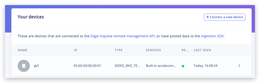
Edge Impulse can ingest data from any device - including embedded devices that you already have in production. See the documentation for the Ingestion service for more information.
2. Collecting your first data
With your device connected we can collect some data. In the studio go to the Data acquisition tab. This is the place where all your raw data is stored, and - if your device is connected to the remote management API - where you can start sampling new data.
Under Record new data, select your device, set the label to idle, the sample length to 5000, the sensor to Built-in accelerometer and the frequency to 62.5Hz. This indicates that you want to record data for 10 seconds, and label the recorded data as idle. You can later edit these labels if needed.
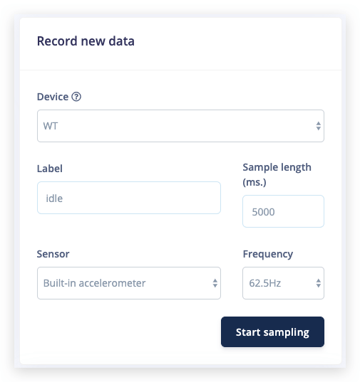
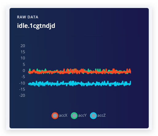
After you click Start sampling move your device up and down in a continuous motion. In about twelve seconds the device should complete sampling and upload the file back to Edge Impulse. You see a new line appear under 'Collected data' in the studio. When you click it you now see the raw data graphed out. As the accelerometer on the development board has three axes you'll notice three different lines, one for each axis.
It's important to do continuous movements as we'll later slice up the data in smaller windows.
Machine learning works best with lots of data, so a single sample won't cut it. Now is the time to start building your own dataset. For example, use the following three classes, and record around 3 minutes of data per class:
- Idle - just sitting on your desk while you're working.
- Wave - waving the device from left to right.
- Circle - drawing circles.
Make sure to perform variations on the motions. E.g. do both slow and fast movements and vary the orientation of the board. You'll never know how your user will use the device. It's best to collect samples of ~10 seconds each.
3. Designing an impulse
With the training set in place you can design an impulse. An impulse takes the raw data, slices it up in smaller windows, uses signal processing blocks to extract features, and then uses a learning block to classify new data. Signal processing blocks always return the same values for the same input and are used to make raw data easier to process, while learning blocks learn from past experiences.
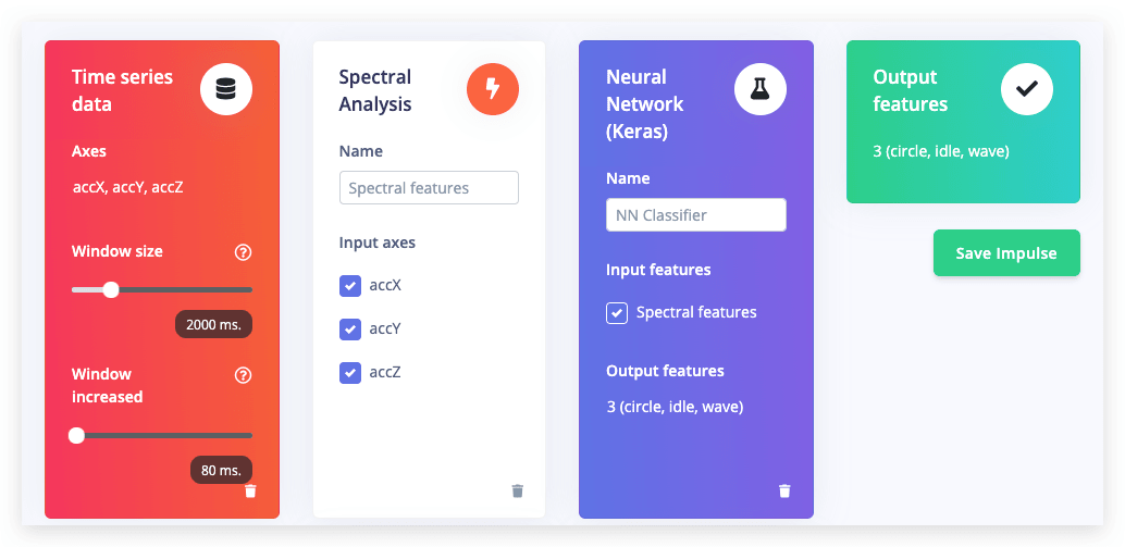
For this tutorial we'll use the 'Spectral analysis' signal processing block. This block applies a filter, performs spectral analysis on the signal, and extracts frequency and spectral power data. Then we'll use a 'Neural Network' learning block, that takes these spectral features and learns to distinguish between the three (idle, circle, wave) classes.
In the studio go to Create impulse, set the window size to 2000 (you can click on the 2000 ms. text to enter an exact value), the window increase to 80, and add the Spectral Analysis and Neural Network (Keras) blocks. Then click Save impulse.
Configuring the spectral analysis block
To configure your signal processing block, click Spectral features in the menu on the left. This will show you the raw data on top of the screen (you can select other files via the drop down menu), and the results of the signal processing through graphs on the right. For the spectral features block you'll see the following graphs:
- After filter - the signal after applying a low-pass filter. This will remove noise.
- Frequency domain - the frequency at which signal is repeating (e.g. making one wave movement per second will show a peak at 1 Hz).
- Spectral power - the amount of power that went into the signal at each frequency.
A good signal processing block will yield similar results for similar data. If you move the sliding window (on the raw data graph) around, the graphs should remain similar. Also, when you switch to another file with the same label, you should see similar graphs, even if the orientation of the device was different.
Once you're happy with the result, click Save parameters. This will send you to the Feature generation screen. In here you'll:
- Split all raw data up in windows (based on the window size and the window increase).
- Apply the spectral features block on all these windows.
Click Generate features to start the process.
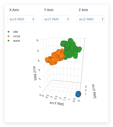
Afterwards the Feature explorer will load. This is a plot of all the extracted features against all the generated windows. You can use this graph to compare your complete data set. E.g. by plotting the height of the first peak on the X-axis against the spectral power between 0.5 Hz and 1 Hz on the Y-axis. A good rule of thumb is that if you can visually separate the data on a number of axes, then the machine learning model will be able to do so as well.
Configuring the neural network
With all data processed it's time to start training a neural network. Neural networks are a set of algorithms, modeled loosely after the human brain, that are designed to recognize patterns. The network that we're training here will take the signal processing data as an input, and try to map this to one of the three classes.
So how does a neural network know what to predict? A neural network consists of layers of neurons, all interconnected, and each connection has a weight. One such neuron in the input layer would be the height of the first peak of the X-axis (from the signal processing block); and one such neuron in the output layer would be wave (one the classes). When defining the neural network all these connections are intialized randomly, and thus the neural network will make random predictions. During training we then take all the raw data, ask the network to make a prediction, and then make tiny alterations to the weights depending on the outcome (this is why labeling raw data is important).
This way, after a lot of iterations, the neural network learns; and will eventually become much better at predicting new data. Let's try this out by clicking on NN Classifier in the menu.
Set Number of training cycles to 1.. This will limit training to a single iteration. And then click Start training.
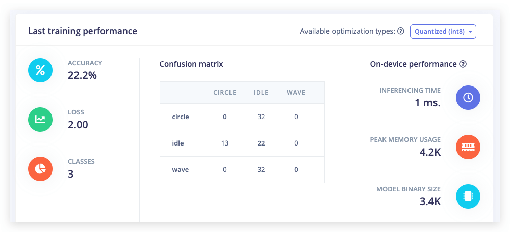
Now change Number of training cycles to 2 and you'll see performance go up. Finally, change Number of training cycles to 100 or more and let training finish. You've just trained your first neural network!
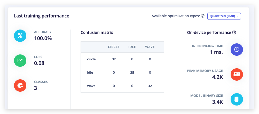
You might end up with a 100% accuracy after training for 100 training cycles. This is not necessarily a good thing, as it might be a sign that the neural network is too tuned for the specific test set and might perform poorly on new data (overfitting). The best way to reduce this is by adding more data or reducing the learning rate.
4. Classifying new data
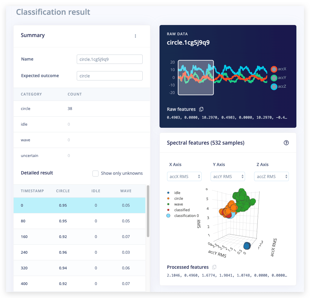
From the statistics in the previous step we know that the model works against our training data, but how well would the network perform on new data? Click on Live classification in the menu to find out. Your device should (just like in step 2) show as online under Classify new data. Set the Sample length to 5000 (5 seconds), click Start sampling and start doing movements. Afterwards you'll get a full report on what the network thought that you did.
If the network performed great, fantastic! But what if it performed poorly? There could be a variety of reasons, but the most common ones are:
- There is not enough data. Neural networks need to learn patterns in data sets, and the more data the better.
- The data does not look like other data the network has seen before. This is common when someone uses the device in a way that you didn't add to the test set. You can add the current file to the test set by clicking, then selecting Move to training set. Make sure to update the label under
Data acquisitionbefore training. - The model has not been trained enough. Up the number of epochs to
200and see if performance increases (the classified file is stored, and you can load it throughClassify existing validation sample). - The model is overfitting and thus performs poorly on new data. Try reducing the learning rate or add more data.
- The neural network architecture is not a great fit for your data. Play with the number of layers and neurons and see if performance improves.
As you see there is still a lot of trial and error when building neural networks, but we hope the visualizations help a lot. You can also run the network against the complete validation set through Model validation. Think of the model validation page as a set of unit tests for your model!
With a working model in place we can look at places where our current impulse performs poorly...
5. Anomaly detection
Neural networks are great, but they have one big flaw. They're terrible at dealing with data they have never seen before (like a new gesture). Neural networks cannot judge this, as they are only aware of the training data. If you give it something unlike anything it has seen before it'll still classify as one of the three classes.
Let's look at how this works in practice. Go to Live classification and record some new data, but now vividly shake your device. Take a look and see how the network will predict something regardless.
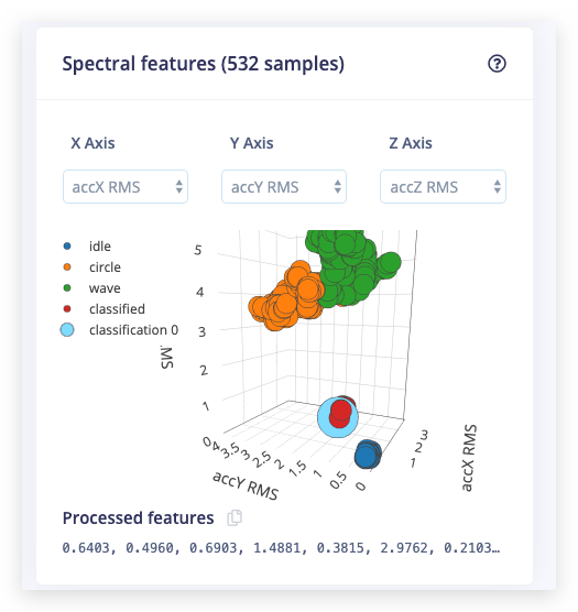
So... how can we do better? If you look at the feature explorer on the accX RMS, accY RMS and accZ RMS axes, you should be able to visually separate the classified data from the training data. We can use this to our advantage by training a new (second) network that creates clusters around data that we have seen before, and compares incoming data against these clusters. If the distance from a cluster is too large you can flag the sample as an anomaly, and not trust the neural network.
To add this block go to Create impulse, click Add learning block, and select K-means Anomaly Detection. Then click Save impulse.
To configure the clustering model click on Anomaly detection in the menu. Here we need to specify:
- The number of clusters. Here use
32. - The axes that we want to select during clustering. As we can visually separate the data on the accX RMS, accY RMS and accZ RMS axes, select those.
Click Start training to generate the clusters. You can load existing validation samples into the anomaly explorer with the dropdown menu.
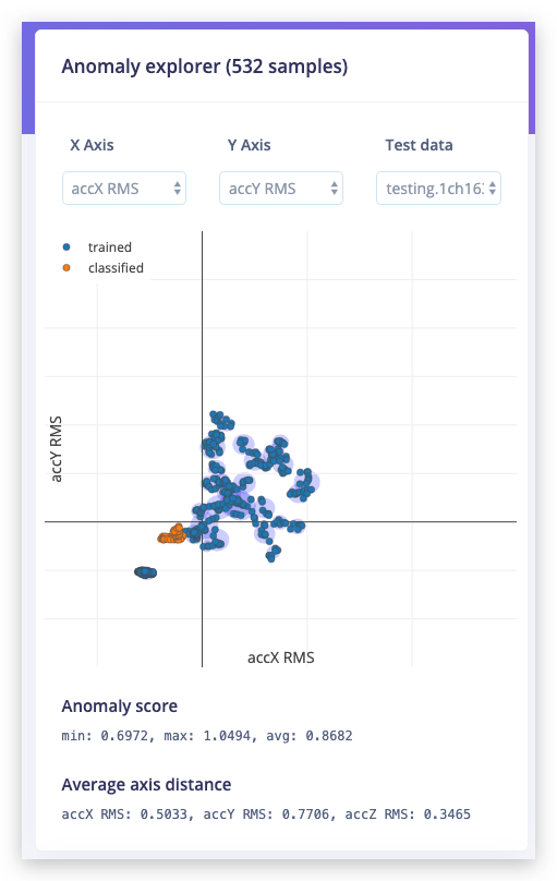
Known clusters in blue, the shake data in orange. It's clearly outside of any known clusters and can thus be tagged as an anomaly.
The anomaly explorer only plots two axes at the same time. Under average axis distance you see how far away from each axis the validation sample is. Use the dropdown menu's to change axes.
6. Deploying back to device
With the impulse designed, trained and verified you can deploy this model back to your device. This makes the model run without an internet connection, minimizes latency, and runs with minimum power consumption. Edge Impulse can package up the complete impulse - including the signal processing code, neural network weights, and classification code - up in a single C++ library that you can include in your embedded software.
After clicking on Deployment tab, choose Arduino library and download it. Extract the archive and place it in your Arduino libraries folder. Open Arduino IDE and choose Examples-> name of your project Inferencing Edge Impulse - > nano_ble33_sense_accelerometer sketch. Our board is similar to Arduino Nano BLE33 Sense, but uses different accelerometer (LIS3DHTR instead of LSM9DS1), so we will need to change the data acquisition section accordingly. Also, since Wio Terminal has an LCD screen, we're going to display name of the detected class if this class confidence value is above threshold. First change the header
#include <Arduino_LSM9DS1.h>
to
#include"LIS3DHTR.h"
#include"TFT_eSPI.h"
LIS3DHTR<TwoWire> lis;
TFT_eSPI tft;
Then change initialization in setup function
    if (!IMU.begin()) {
        ei_printf("Failed to initialize IMU!\r\n");
    }
    else {
        ei_printf("IMU initialized\r\n");
    }
to
    tft.begin();
    tft.setRotation(3);
    tft.fillScreen(TFT_WHITE);

 lis.begin(Wire1);

    if (!lis.available()) {
    Serial.println("Failed to initialize IMU!");
    while (1);
    }
    else {
        ei_printf("IMU initialized\r\n");
    }
    lis.setOutputDataRate(LIS3DHTR_DATARATE_100HZ); // Setting output data rage to 25Hz, can be set up tp 5kHz
    lis.setFullScaleRange(LIS3DHTR_RANGE_16G); // Setting scale range to 2g, select from 2,4,8,16g
We do data collection and inference within loop function, here is where we need to change data acquisition with LSM9DS1 to data acquisition function for LIS3DHTR
IMU.readAcceleration(buffer[ix], buffer[ix + 1], buffer[ix + 2]);
to
lis.getAcceleration(&buffer[ix], &buffer[ix + 1], &buffer[ix + 2]);
And then to display the class name on the LCD screen, after
#if EI_CLASSIFIER_HAS_ANOMALY == 1
    ei_printf("    anomaly score: %.3f\n", result.anomaly);
#endif
add the following code block, in which we check confidence values of every class and if one of them is higher than threshold, change the color of the screen and display that classes name.
   if (result.classification[1].value > 0.7) {
    tft.fillScreen(TFT_PURPLE);
    tft.setFreeFont(&FreeSansBoldOblique12pt7b);
    tft.drawString("Wave", 20, 80);
    delay(1000);
    tft.fillScreen(TFT_WHITE);
   }

   if (result.classification[2].value > 0.7) {
    tft.fillScreen(TFT_RED);
    tft.setFreeFont(&FreeSansBoldOblique12pt7b);
    tft.drawString("Circle", 20, 80);
    delay(1000);
    tft.fillScreen(TFT_WHITE);
   }
Then compile and upload - open the serial monitor and perform one the gestures! You will be able to see the inference results displayed on the Serial monitor and also on LCD screen.
7. Conclusion
Machine learning is a super interesting field: it allows you to build complex systems that learn from past experiences, automatically find patterns in sensor data, and search for anomalies without explicitly programming things out. We think there's a huge opportunity for machine learning on embedded systems. There are huge amounts of sensor data currently collected, but 99% of this data is currently discarded due to cost, bandwidth or power constraints.
Edge Impulse helps you unlock this data. By processing data directly on the device you no longer have to send raw data to the cloud, but can draw conclusions directly where it matters. We can't wait to see what you will build!