reBot Arm B601-DM Pinocchio & MeshCat

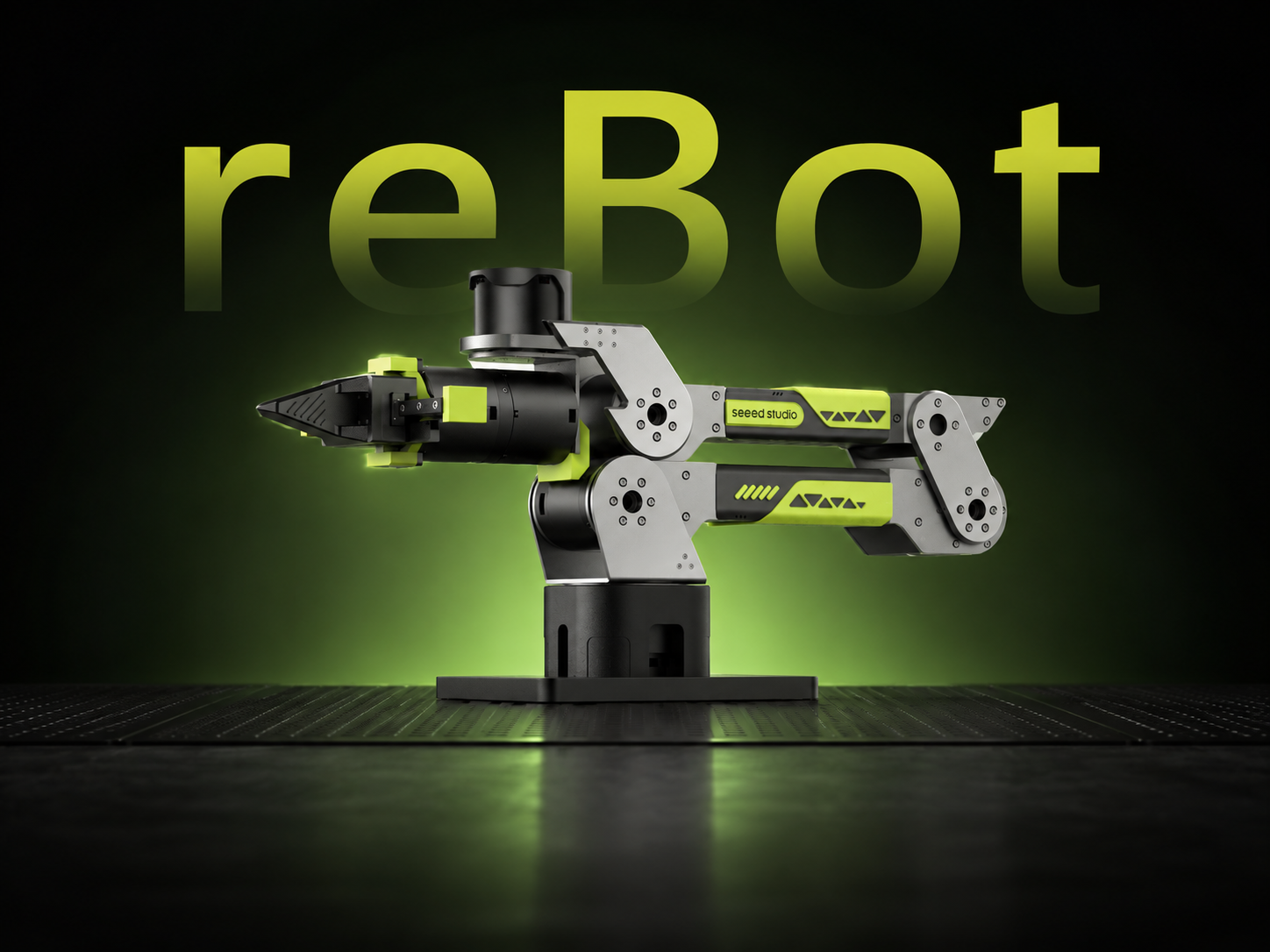
6-DOF Robotic Arm · Multi-Motor Support · Kinematics Solver · Trajectory Planning · Fully Open Source

tip

This example code can be used to control the robotic arm motors or poses, including single motor control, forward/inverse kinematics control and testing, arm zero position setting and motor angle reading, MeshCat visualization system, and more.

Pinocchio is an open-source library for robotics dynamics analysis and optimization. It provides efficient forward/inverse kinematics, dynamics calculations, and trajectory planning capabilities.

MeshCat is a web-based 3D visualization tool that can display robot status and motion trajectories in real-time.

This project combines Pinocchio's powerful computing capabilities with MeshCat's intuitive visualization, providing a complete set of kinematic analysis and debugging tools for reBot Arm B601-DM.

Star on GitHub4.2K

Project Features

Complete Kinematic Analysis Supports Forward Kinematics (FK) and Inverse Kinematics (IK) calculations, able to solve the robot arm's end-effector pose in real-time.
Real-time 3D Visualization Displays robot arm status and motion trajectories in real-time through MeshCat in the browser, no additional software required.
Trajectory Planning and Tracking Implements SE(3) geodesic trajectory planning, supporting CLIK (Closed-Loop Inverse Kinematics) tracking control.
Gravity Compensation Control Calculates joint gravity torque based on Pinocchio dynamics model, achieving the "floating" effect of the robot arm.
Open Source & Extensible All code is open source, supporting users to customize control algorithms and visualization effects according to their needs.

Specifications

The hardware for this tutorial is provided by Seeed Studio

Parameter	Specification
Robot Arm Model	reBot Arm B601-DM
Degrees of Freedom	6-DOF + Gripper
Motor Model	Damiao DM4340 / DM4310
Communication Method	CAN Bus via USB-CAN Adapter
Operating Voltage	24V DC
Control Method	PC
Recommended Operating Temperature Range	0°C ~ 40°C

Bill of Materials (BOM)

Component	Quantity	Included
reBot Arm B601-DM Robotic Arm	1	✅
USB2CAN Serial Bridge	1	✅
Power Adapter (24V)	1	✅
USB-C Cable	1	✅
Gripper	1	✅

Environment Requirements

Prerequisite — Complete the Arm Quick Start First

Before proceeding with this tutorial, you must finish the reBot Arm B601-DM Quick Start document end-to-end, including:

Hardware unboxing, wiring, and power-on checklist
Serial / CAN device permission (sudo chmod 666 /dev/ttyACM0 or /dev/can0)
Zero calibration of all joints (2_zero_and_read.py) and verifying the arm can be commanded in MIT / POS_VEL mode

This tutorial assumes the arm is already responsive on the bus, joints are zeroed, and the operator is familiar with the relevant safety limits. Skipping the Quick Start can lead to mis-configured motors, stalled joints, or arm drops.

Item	Requirement
Python	3.10+
Operating System	Ubuntu (Ubuntu 24.04 LTS recommended)
Communication Interface	USB2CAN Serial Bridge or CAN Interface

Installation Steps

Install uv (if not installed)

Step 1

curl -LsSf https://astral.sh/uv/install.sh | sh

After installation, run the following command to verify that uv is available:

uv --version

If the installation succeeded, you should see output similar to the following (the version and platform may differ):

uv 0.11.31 (x86_64-unknown-linux-gnu)

Sync Environment (Install All Dependencies)

Step 2

git clone https://github.com/Seeed-Projects/reBotArm_control_py.git
cd reBotArm_control_py
uv sync

tip

uv sync will automatically create a virtual environment (if it doesn't exist) and install all dependencies according to pyproject.toml and uv.lock.

Tuning MIT / POS_VEL Controller Parameters

This section explains how to modify the controller parameters for each joint of the arm under MIT mode and POS_VEL mode, and how to make the changes take effect.

This section only covers "where / how to change", not "what value to use"

Suitable parameters can only be obtained through on-hardware tuning. This section only covers: where the parameters live, what each field controls, and how to make the changes effective and verify them. For specific tuning strategies (e.g., trial-and-error, Ziegler‑Nichols), please refer to general motor control references.

Configuration File Location

Hardware version	Motor config file	Switch entry
reBot Arm B601-DM (this document)	`config/rebotarm_dm.yaml`	Set `hardware_yaml: "rebotarm_dm.yaml"` in `config/rebotarm.yaml`
reBot Arm B601-RS	`config/rebotarm_rs.yaml`	Set `hardware_yaml: "rebotarm_rs.yaml"` in `config/rebotarm.yaml`

Do not edit rebotarm.yaml directly

That file only contains a single line hardware_yaml: ...; all motor parameters live in rebotarm_dm.yaml / rebotarm_rs.yaml.

Configuration File Structure

Each joint has its own entry, grouped by control mode:

joints:
  - name: joint1
    motor_id: 0x01
    feedback_id: 0x11
    model: "4340P"
    vendor: "damiao"
    MIT:
      kp: 120.0
      kd: 8.0
    POS_VEL:
      vel_kp: 0.0125
      vel_ki: 0.004
      pos_kp: 150.0
      pos_ki: 0.5
      vlim: 5.0
  # ... joint2 ~ joint6 follow the same structure ...

How to locate:

By joint name: to modify a joint, find the - name: jointX block;
By mode: under that joint, MIT: holds MIT mode parameters, POS_VEL: holds POS_VEL mode parameters;
Current mode determines which set is sent: the script switches modes via mode mit / mode posvel; the motor actually receives the parameters under the corresponding sub-block.

MIT Mode Field Meanings

Field	Role
`kp`	Position-loop proportional gain: the "stiffness" of tracking the target position.
`kd`	Velocity-loop damping gain: suppresses oscillations caused by position error.

POS_VEL Mode Field Meanings

Field	Role
`vel_kp`	Velocity-loop proportional gain.
`vel_ki`	Velocity-loop integral gain.
`pos_kp`	Position-loop proportional gain.
`pos_ki`	Position-loop integral gain (only present in some vendor configs).
`vlim`	Speed limit, caps the maximum motion speed.

Field definitions differ across vendors

Damiao (DM) and Robostride (RS) motors use different protocol-layer units, so the same field name has no cross-vendor comparability. Modifying RS's vel_kp and modifying DM's vel_kp mean different things. Please interpret each YAML according to its own field order, do not compare values across config files.

Limit the Test Scope Before Tuning

Large kp / kd changes across several joints can cause immediate oscillation, overcurrent, or hard-stop collisions if any joint direction or sign is wrong. Before tuning, clear the arm's workspace and plan to test one joint and one mode at a time, in small steps.

Editing Procedure

Stop any running script. The motor is enabled when you edit YAML, changes do not take effect immediately, and inconsistent behavior is easy to trigger.
Edit the corresponding YAML file:
```
# Example for DM
vim config/rebotarm_dm.yaml
```
- Only change the joint you need to tune (e.g., joint1); leave unrelated joints alone;
- Within one joint, only change the mode you need to tune (MIT or POS_VEL); do not modify the other mode's fields without reason.
Preserve YAML indentation: 2 spaces per level, keys separated from values by :. Wrong indentation causes yaml.safe_load parsing to fail, and all parameters will fall back to defaults.
Restart the script after saving. The YAML is read once at script startup; runtime edits do not take effect immediately.
Single-joint verification: use a script like 3_mit_control.py (MIT) / 4_pos_vel_control.py (POS_VEL) to verify the change with a small single-joint motion before doing a full-arm test.

Verifying the Change Took Effect

Runtime observation: enable the motor in 3_mit_control.py / 4_pos_vel_control.py and check state; if parameters look unchanged or the motor behaves exactly as before, the YAML was edited incorrectly or got overridden by defaults.
YAML self-check: parse it directly with Python and print one joint's fields to confirm the values match what you just wrote:
```
uv run python -c "import yaml; print(yaml.safe_load(open('config/rebotarm_dm.yaml'))['joints'][0])"
```
Quick rollback: git checkout config/rebotarm_dm.yaml restores the repository defaults.

Debug Tools Introduction

Permission Settings

Before running hardware control examples, you need to set device permissions:

# Set serial device permissions (Damiao USB2CAN)
sudo chmod 666 /dev/ttyACM0

# Or set CAN device permissions (e.g., can0)
sudo chmod 666 /dev/can0

Debugging Tools (use only when an exception occurs)

Single Motor Control Console (0x01damiao_test.py)

Direct single motor testing using the motorbridge SDK.

How to Run:

uv run python example/0x01damiao_test.py

Interactive Commands:

Command	Description
`enable` / `disable`	Enable/Disable motor
`set_zero`	Set zero position
`state`	View status
`ping`	Ping motor to get response
`clear_error`	Clear motor errors
`mode <mit/posvel/vel>`	Switch control mode
`mit <pos> [vel] [kp] [kd]`	MIT mode command
`posvel <pos> [vlim]`	POS_VEL mode command
`vel <velocity>`	Pure velocity mode command
`read_param <id> [type]`	Read motor parameters
`write_param <id> <value> [type]`	Write motor parameters
`loop`	Enter loop control mode
`q` / `quit`	Quit

Zero Calibration and Angle Monitoring (2_zero_and_read.py)

Automatically set all joint zeros and display joint angles in real-time.

How to Run:

uv run python example/2_zero_and_read.py

# Example Output
-0.12  +0.23  -6.42  +41.74  -0.45  -0.01  -0.01

MIT Control Mode (alternative on reBot DM, view on demand — POS_VEL is recommended)

Demo 3 · 3_mit_control.py

Optional — MIT Is the Alternative Mode on DM

For the reBot Arm B601-DM, POS_VEL (Position‑Velocity) is generally the more appropriate joint-control mode; the Damiao motor protocol natively supports position‑velocity hybrid control with built-in speed limiting. MIT mode usually requires more careful kp / kd tuning.

This example is not required to complete the tutorial. Unless you specifically need to debug MIT mode, skip this example and use the POS_VEL example below. If your goal is smooth end-effector motion along a planned path, go directly to Smooth Trajectory IK Control (8_arm_traj_control.py).

Input target angles for all joints to complete motor control in MIT control mode, typically used for force control, impedance control, or scenarios requiring high dynamic response.

Before Running — This Example Has No Smooth Trajectory Planning

This example sends target joint angles directly to the motors, with no path or velocity planning. A large target change can cause sudden high-speed motion and trigger overcurrent protection.

Run it only when you need to verify low-level MIT joint control. Start by moving one joint by only 5–10 degrees, then increase the change gradually after confirming the response and direction;
If you need a complete smooth trajectory, skip this example and go to Smooth Trajectory IK Control (8_arm_traj_control.py);
Clear the arm's workspace before running and make sure you can cut power immediately.

Expand Run Instructions (Optional)

How to Run:

uv run python example/3_mit_control.py
> 30 0 0 0 0 0 0 # Control motor 1 to rotate 30 degrees
> state
  pos (deg): ['+29.99', '+0.00', '-45.00', '+0.00', '+0.00', '+0.00']
> q # Exit system

Position-Velocity Control Mode

Demo 4 · 4_pos_vel_control.py

Enter target angles for all joints to control the motors in POS_VEL (Position-Velocity) hybrid mode. Damiao's built-in speed limiting can reduce the impact of target changes, but this example itself does not provide complete smooth trajectory planning.

Optional — Speed Limiting Is Not Complete Trajectory Planning

Although POS_VEL is the recommended joint-control mode for DM, this example still updates joint position targets directly and does not plan the intermediate path. A large target change can still cause sudden motion, collision, or overcurrent.

This example is not required to complete the tutorial. If you only need smooth end-effector motion, skip this example and go directly to Smooth Trajectory IK Control (8_arm_traj_control.py);
When verifying POS_VEL joint control, start by moving one joint by only 5–10 degrees, then increase the target change gradually;
Clear the arm's workspace before running and make sure you can cut power immediately.

Expand Run Instructions (Optional)

How to Run:

uv run python example/4_pos_vel_control.py
> 30 0 0 0 0 0 0 # Control motor 1 to rotate 30 degrees
> state
  pos (deg): ['+29.99', '+0.00', '-45.00', '+0.00', '+0.00', '+0.00']
> q # Exit system

Kinematics Testing

Forward Kinematics Testing

Demo 5 · 5_fk_test.py

Calculate end-effector pose based on joint angles.

Input: 6 joint angles (degrees)

Output:

End-effector position (X, Y, Z) — Unit: meters
Rotation matrix (3×3)
Euler angles (roll/pitch/yaw) — Unit: degrees

Example:

uv run python example/5_fk_test.py
> 0 0 0 0 0 0
====================================================
  Result / Result
====================================================
  Joint angles (deg): [0. 0. 0. 0. 0. 0.]
  End-effector position (m):
    X = +0.260306
    Y = +0.000000
    Z = +0.191701
  Rotation matrix (R_world^end):
    [+1.000000  +0.000000  -0.000007]
    [+0.000000  +1.000000  +0.000100]
    [+0.000007  -0.000100  +1.000000]
  Euler XYZ (roll, pitch, yaw) [deg]:
    roll   = -0.0057
    pitch  = -0.0004
    yaw    = +0.0000

Inverse Kinematics Testing

Demo 6 · 6_ik_test.py

Solve joint angles based on desired end-effector pose.

Input Format:

Position only: <x> <y> <z> (meters)
Position + Orientation: <x> <y> <z> <roll> <pitch> <yaw> (degrees)

Example:

uv run python example/6_ik_test.py

# Usage A
> 0.28 0 0.3  # Position only
====================================================
  Result / Result
====================================================
  Target position : [+0.2800, +0.0000, +0.3000] m
  Converged : Yes
  Iterations: 2000
  Position error: 5.62e-17 m
  Joint angles (deg) [first 6 control joints]:
    joint1     =  -0.0003 deg  (-0.0000 rad)
    joint2     = -22.9687 deg  (-0.4009 rad)
    joint3     = -24.2191 deg  (-0.4227 rad)
    joint4     =  +1.2508 deg  (+0.0218 rad)
    joint5     =  -0.0003 deg  (-0.0000 rad)
    joint6     =  +0.0057 deg  (+0.0001 rad)

# Usage B
> 0.28 0 0.3 0 1 0       # Position + Orientation
====================================================
  Result / Result
====================================================
  Target position   : [+0.2800, +0.0000, +0.3000] m
  Target orientation : [+0.00, +1.00, +0.00] deg
  Converged  : Yes
  Iterations: 2000
  Position error: 6.28e-17 m
  Joint angles (deg) [first 6 control joints]:
    joint1     =  -0.0003 deg  (-0.0000 rad)
    joint2     = -23.3968 deg  (-0.4084 rad)
    joint3     = -25.3018 deg  (-0.4416 rad)
    joint4     =  +2.9054 deg  (+0.0507 rad)
    joint5     =  -0.0003 deg  (-0.0000 rad)
    joint6     =  +0.0057 deg  (+0.0001 rad)

Inverse Kinematics Control in MIT Mode

Demo 7 · 7_arm_ik_control.py

Use inverse kinematics (IK) in MIT mode to specify the 3D coordinates (X, Y, Z) and orientation (Euler angles) where the robotic arm end-effector should move.

Input Format:

Position only: <x> <y> <z> (meters)
Position + Orientation: <x> <y> <z> <roll> <pitch> <yaw> (degrees)
Input state: View current actual radian values of each joint.
Input end_state: View current end-effector actual coordinates (m) and Euler angles (rad) in space.

Optional — This Example Has No Smooth Trajectory Planning

This example sends the IK solution directly as the joint target, with no path or velocity planning. A large target-pose change can cause sudden high-speed motion and trigger overcurrent protection.

This example is not required to complete the tutorial. In most cases, skip this example and use the next section, Smooth Trajectory IK Control (8_arm_traj_control.py), which includes minimum-jerk acceleration/deceleration planning;
Run it only when you need to compare or debug IK control without trajectory planning. Keep the first target within 5–10 cm of the current end-effector position;
Before running, confirm the target pose is reachable, clear the workspace of people and obstacles, and make sure you can cut power immediately.

Expand Run Instructions (Optional)

How to Run:

uv run python example/7_arm_ik_control.py

#Usage A
> 0.3 0.0 0.4 # Position only (orientation defaults to 0), move the arm end-effector to 0.3 meters forward and 0.4 meters above.

#Usage B
> 0.3 0.0 0.4 0.0 0.0 0.5 # Control both position and orientation: move to the specified position while rotating the wrist yaw angle by 0.5 radians.

> ctrl + c # Return to zero position and exit system

Inverse Kinematics Control with Smooth Trajectory

Demo 8 · 8_arm_traj_control.py

Use inverse kinematics (IK) in MIT mode to automatically plan a uniform or smooth acceleration/deceleration motion trajectory within the target time, avoiding severe joint vibration.

Input Format:

Position only: <x> <y> <z> (meters)
Position + Orientation: <x> <y> <z> <roll> <pitch> <yaw> (degrees)
Position + Orientation + Time (default 2.0): <x> <y> <z> <roll> <pitch> <yaw> <time> (degrees)
Input state: View current actual radian values of each joint.
Input end_state: View current end-effector actual coordinates (m) and Euler angles (rad) in space.

How to Run:

uv run python example/8_arm_traj_control.py

#Usage A
> 0.3 0.0 0.4 # Position only, orientation defaults to 0, default movement time is 2.0 seconds

#Usage B
> 0.3 0.0 0.4 0.0 0.0 0.5 # Control both position and orientation: move to the specified position while rotating the wrist yaw angle by 0.5 radians, default movement time is 2.0 seconds

#Usage C
> 0.3 0.0 0.4 0.0 0.0 0.0 5.0 # Move the arm to the specific position and specify 5.0 seconds to slowly move there. (Note: If entering time, the preceding orientation parameters 0 0 0 cannot be omitted)

> ctrl + c # Return to zero position and exit system

What if I observe pose deviation?

If you notice that the read end-effector pose differs from the commanded target pose, and the pose itself is reachable (not outside workspace, not at a singularity), the problem is likely in your MIT / POS_VEL controller parameters. In that case, please refer to the earlier Tuning MIT / POS_VEL Controller Parameters section and manually tune kp / kd etc. using the "single joint, mode by mode, small steps" approach; once tuned, return to this example to verify.

Gravity Compensation Testing

Gravity Compensation Control — Basic Version

Demo 9 · 9_gravity_compensation.py

Use the Pinocchio dynamics model to compensate for joint gravity.

Control Law:

tau = g(q)          — Gravity feedforward
pos = current motor position   — Joint position follows current position
kp = 2,  kd = 1     — Unified stiffness/damping for all joints

Expected Behavior:

The arm can "float" at any pose
Won't fall due to its own weight when released
Can be manually moved to any position

Normal Exit Performs a Safe Return Home

When you stop the script normally with Ctrl+C, it first stops gravity-compensation control and holds the current pose with stiff gains and gravity feedforward. It then returns the arm to zero through a minimum-jerk trajectory; only after homing completes does it disconnect and disable the motors.

Automatic homing depends on normal program execution, communication, and power. Keep people and obstacles outside the arm's workspace and be ready to support the arm during homing. A communication failure, unexpected power loss, or forced termination may prevent the protection sequence from completing; cut power immediately if abnormal motion occurs.

How to Run:

uv run python example/9_gravity_compensation.py

Output:

Real-time display of desired torque for each joint (N·m)
Press Ctrl+C to stop and disconnect

Adjusting Individual Joint Compensation

If some joints are under-compensated or over-compensated due to structural friction or assembly differences, you can apply additional scaling to the corresponding element of the tau_g array in the code:

tau_g[x] *= y  # x is the joint motor id, y is the compensation factor, usually starting from 1
# This compensation is generally only used for joints 2 and 3

For example, tau_g[2] *= 1.2 means increasing the gravity compensation torque of joint 2 by 20%. It is recommended to adjust item by item based on the actual floating effect to avoid making excessively large changes at once.

Gravity Compensation Control — End-Effector Velocity Lock Version

Demo 10 · 10_gravity_compensation_lock.py

Based on the basic gravity compensation, adds end-effector velocity detection and joint angle locking mechanism.

Control Law:

tau = g(q) + integral_term    — Gravity feedforward + integral term
pos = q_target                 — Target joint angle (locked or updated)
kp = 8.0,  kd = 1.0           — Enhanced stiffness/damping

Lock Logic:

When end linear velocity ||v_ee|| < 0.04 m/s and angular velocity ||w_ee|| < 0.08 rad/s:
- Target joint angle q_target remains locked
- Robotic arm locks in current position
When end velocity exceeds threshold:
- q_target updates to current joint angle
- Allows manual pushing to change position

Expected Behavior:

Robotic arm locks in current position, requiring force to change target angle
More stable than basic version, suitable for scenarios requiring pose maintenance

Normal Exit Performs a Safe Return Home

How to Run:

uv run python example/10_gravity_compensation_lock.py

Output:

Real-time display of lock status (LOCKED / UPDATE)
End linear velocity, angular velocity
Gravity compensation torque for each joint (N·m)
Press Ctrl+C to stop and disconnect

Adjusting Individual Joint Compensation

tau_g[x] *= y  # x is the joint motor id, y is the compensation factor, usually starting from 1
# This compensation is generally only used for joints 2 and 3

Safety Test Configuration: You can modify the ENABLED_JOINTS list at the top of the script to enable only specified joints for safety testing:

ENABLED_JOINTS = ["joint1"]  # Enable only joint1

Simulation Environment

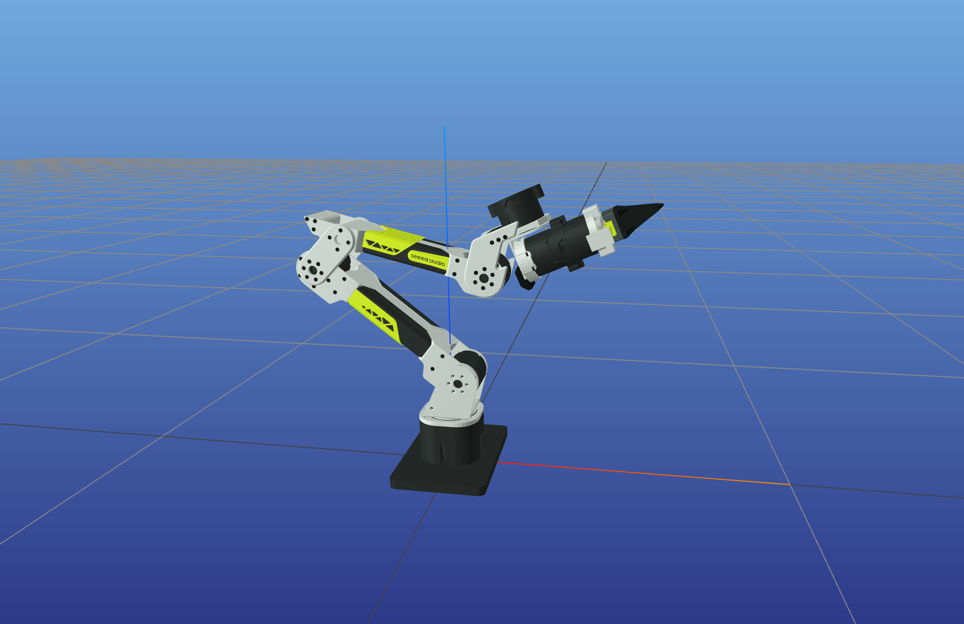
MeshCat simulation of the reBot Arm B601-DM

MeshCat web viewer address

After starting a simulation, the terminal prints the actual access URL. The default is http://127.0.0.1:7000/static/; if the port is occupied, MeshCat automatically tries the next port, so use the URL printed in the terminal.

Forward Kinematics Simulation

Simulation Demo 1 · sim/fk_sim.py

Interactive forward kinematics simulation, visualize robot arm pose by inputting joint angles in MeshCat.

How to Run:

uv run python example/sim/fk_sim.py

Interactive Commands:

Input 6 joint angles (degrees), space separated
Example: 0 0 0 0 0 0
Example: 45 -30 15 -60 90 -180
q/quit/exit: Exit

Features:

Real-time display of end-effector position and orientation
Supports continuous input to test different poses
Formatted pose information output

Inverse Kinematics Simulation

Simulation Demo 2 · sim/ik_sim.py

Interactive inverse kinematics simulation, automatically solve joint angles from target pose and visualize.

How to Run:

uv run python example/sim/ik_sim.py

Input Format:

Position only: x y z (meters)
Position+Orientation: x y z roll pitch yaw (radians)

Example:

> 0.25 0.0 0.25              # Position only
> 0.25 0.0 0.25 0 0 0        # Position+Orientation

Features:

Automatic judgment of IK convergence
Display iteration count and error
Real-time robot pose updates

Trajectory Planning Simulation

Simulation Demo 3 · sim/traj_sim.py

SE(3) geodesic based trajectory planning simulation, including CLIK tracking and MeshCat animation playback.

How to Run:

uv run python example/sim/traj_sim.py

Interactive Commands:

Input: x y z [roll pitch yaw] (meters/radians)
Press Enter to use default configuration
q: Exit

Features:

Plan from current position to target position
Use minimum jerk trajectory profile
Real-time display of trajectory statistics
Complete trajectory animation playback in MeshCat
Display reference path (gray) and actual path (green)

Visualizer Tool

Simulation Demo 4 · sim/visualizer.py

MeshCat visualizer wrapper, providing unified robot display interface.

Main Features:

Load URDF model and display robot
Draw 3D polyline paths (reference/actual)
Display IK target pose (tricolor axes + sphere)
Support joint trajectory animation playback

Usage Example:

from example.sim.visualizer import Visualizer
viz = Visualizer()
viz.update(q)  # Update robot pose
viz.draw_path(points, "path_name", color)  # Draw path

FAQ

Encountering Permission denied error Ensure you have executed sudo chmod 666 /dev/ttyACM0 or sudo chmod 666 /dev/can0 to set device permissions.
IK solving fails or results are abnormal Check if the target pose is within the robot arm's workspace, ensure joint limit configuration is correct.
Gravity compensation effect is not good This may be caused by structural errors and processing accuracy. The gravity compensation of this project depends on URDF and Pinocchio. You can try correcting the URDF to your actual measured parameters (you can ask AI for this step).

Contact

Technical Support: Submit Issue
Project Repository: GitHub
Forum: Seeed Studio Forum

Reference Documents

If this project helps you, please give us a Star!

Project Features​

Specifications​

Bill of Materials (BOM)​

Environment Requirements​

Installation Steps​

Install uv (if not installed)

Sync Environment (Install All Dependencies)

Tuning MIT / POS_VEL Controller Parameters​

Configuration File Location​

Configuration File Structure​

MIT Mode Field Meanings​

POS_VEL Mode Field Meanings​

Editing Procedure​

Verifying the Change Took Effect​

Debug Tools Introduction​

MIT Control Mode (alternative on reBot DM, view on demand — POS_VEL is recommended)

Position-Velocity Control Mode

Kinematics Testing​

Forward Kinematics Testing

Inverse Kinematics Testing

Inverse Kinematics Control in MIT Mode

Inverse Kinematics Control with Smooth Trajectory

Gravity Compensation Testing​

Gravity Compensation Control — Basic Version

Gravity Compensation Control — End-Effector Velocity Lock Version

Simulation Environment​

Forward Kinematics Simulation

Inverse Kinematics Simulation

Trajectory Planning Simulation

Visualizer Tool

FAQ​

Contact​

Reference Documents​

Project Features

Specifications

Bill of Materials (BOM)

Environment Requirements

Installation Steps

Tuning MIT / POS_VEL Controller Parameters

Configuration File Location

Configuration File Structure

MIT Mode Field Meanings

POS_VEL Mode Field Meanings

Editing Procedure

Verifying the Change Took Effect

Debug Tools Introduction

Kinematics Testing

Gravity Compensation Testing

Simulation Environment

FAQ

Contact

Reference Documents