Evo-1 — Lightweight VLA
Evo-1: Lightweight Vision-Language-Action Model with Preserved Semantic Alignment
- Lightweight VLA
- Semantic alignment
- Cross-attention
- Two-stage training
Prerequisites: From Instructions to Actions
What Does a VLA Learn?
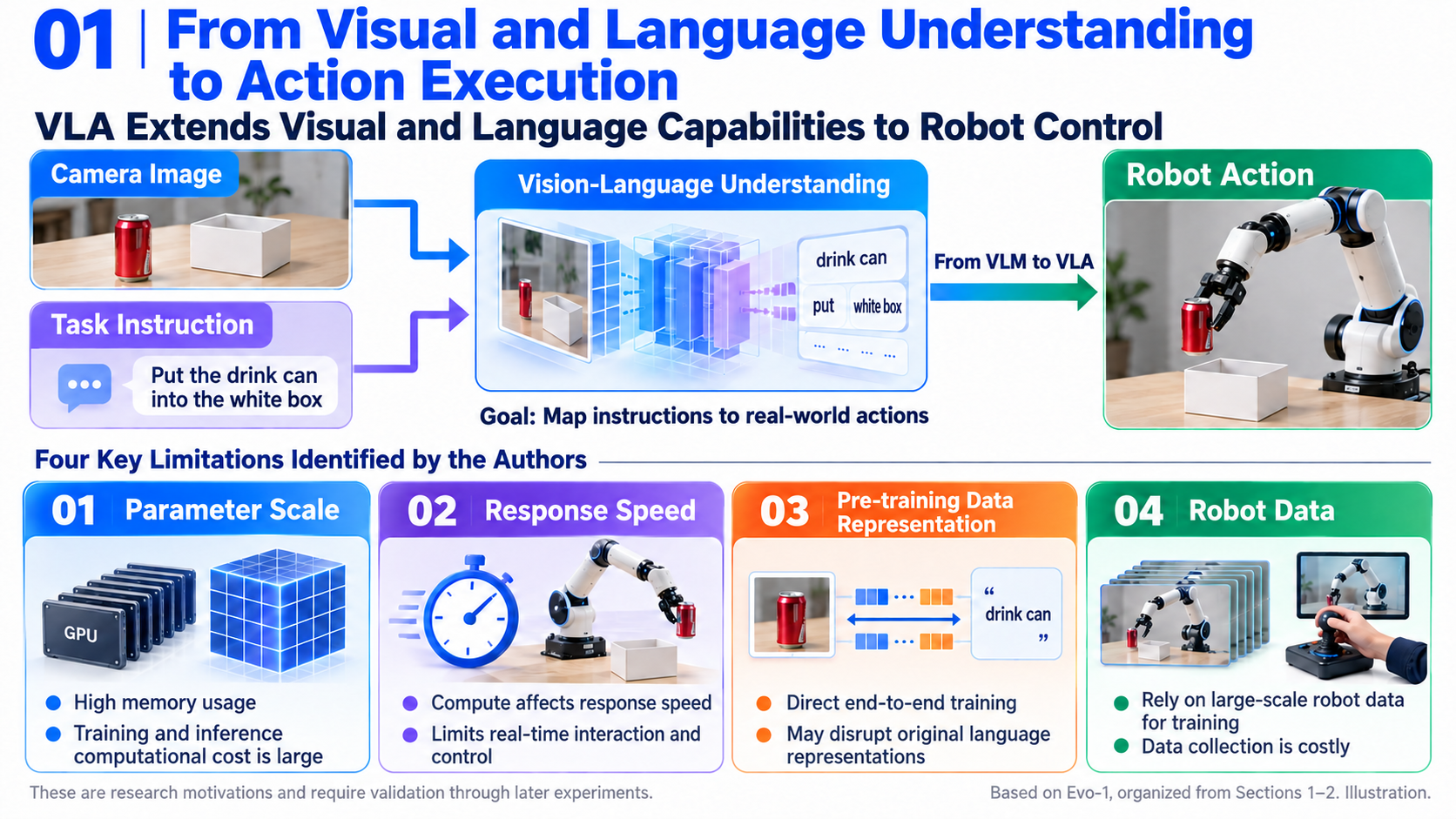
Explanation: Imitation learning teaches the robot how to move in a demonstrated situation. A vision-language-action model adds task text, learning control actions conditioned on both images and instructions.
For the paper's “put the beverage can into the white box” task, teleoperation supplies camera images, robot configurations, and corresponding actions. The model learns their relationship to the task text. At deployment, current images, an instruction, and state produce future actions, rather than just a verbal instruction to pick up the can.
| Concept | Meaning | Example in Evo-1 |
|---|---|---|
| Observation | Information used to assess the environment | Multi-view RGB images; the real xArm6 uses fixed and wrist cameras. |
| Proprioceptive state | Numerical description of the robot itself | Absolute joint angles in the real-robot dataset. |
| Action | Numerical commands for the control interface | Recorded as absolute joint angles on the real system; other platforms use their own action interfaces. |
| Vision-language model (VLM) | Converts images and text into jointly processed features | The InternVL3-1B backbone. |
| Semantic alignment | Preserving correspondence between image content and language meaning | “Beverage can” should relate to the visible can rather than irrelevant background. |
Caution: Preserving alignment is a design goal supported by attention visualizations and task results. It is not a comprehensive evaluation of all language knowledge.
Single-Step Actions and Chunks
Single-step prediction outputs only the current action. Action chunking predicts several future actions jointly. Evo-1's default horizon is 50 steps.
Single-step: current images, instruction, state → aₜ
Action chunking: current images, instruction, state → [aₜ, aₜ₊₁, …, aₜ₊₄₉]
Illustrative example: For one joint, three target angles might be [0.10, 0.12, 0.15] radians. Single-step prediction produces them separately; chunking predicts the sequence together. Actual Evo-1 outputs multidimensional 50-step chunks.
Chunks model continuous trajectories, but the environment can change during execution. The paper does not fully specify how many steps are executed before re-observation, overlap blending, or replanning on every platform. Predicting 50 steps therefore does not imply executing all 50 open-loop, and chunk length does not determine the final control frequency.
Distinguish Three Stages
| Stage | Inputs and operations | Outcome or criterion |
|---|---|---|
| Training | Demonstration images, instructions, states, and actions; noise is added to actions to learn a generation direction. | Model parameters; loss measures direction-prediction error. |
| Inference | Current images, instruction, state, and a newly sampled noisy action chunk. | Generate continuous future actions for execution. |
| Evaluation | Execute under specified tasks and initial conditions. | Task success, plus VRAM and inference-rate measurements on a specified GPU. |
Low training loss does not directly imply high real-task success. The training mechanism and evaluation evidence are discussed separately below.
Abstract: Translation and Commentary
Translation
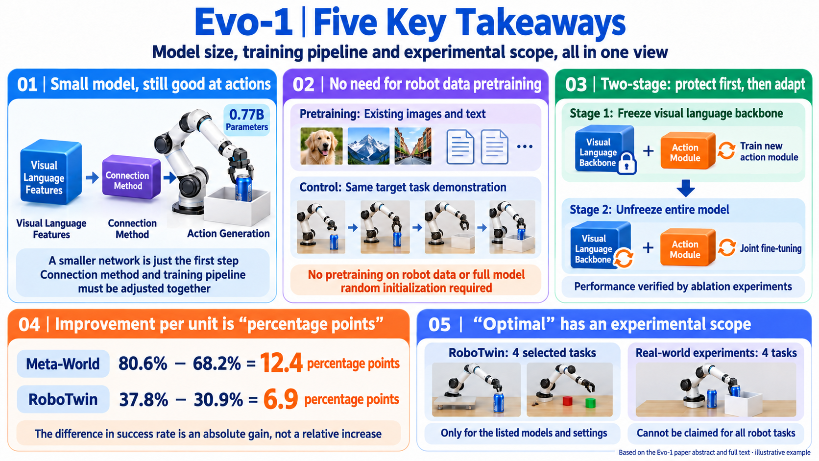
VLAs unify perception, language, and control, enabling diverse tasks through multimodal understanding. However, many have large parameter counts and depend heavily on large-scale robot-data pre-training, increasing training costs and limiting real-time deployment. Some training approaches can also weaken the backbone's perceptual representations, leading to overfitting and poor downstream generalization.
Evo-1 is a lightweight VLA that improves deployment efficiency without robot-data pre-training. It builds on a natively multimodal VLM with a cross-modulated diffusion Transformer and an optimized integration module. A two-stage training process progressively aligns actions with perception while retaining useful VLM representations.
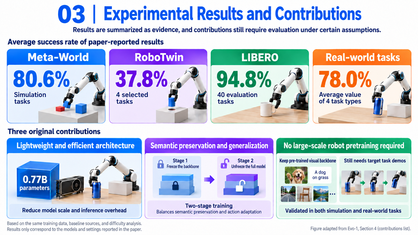
With 770 million parameters, Evo-1 reports state-of-the-art results at publication on Meta-World and RoboTwin, exceeding the compared best results by 12.4 and 6.9 percentage points, and a competitive 94.8% on LIBERO. Real-world evaluation reports 78% average success with fast inference and low memory use, outperforming the compared baselines. Code, data, and weights are released.
Commentary
Introduction and Related Work: Why Change Architecture and Training?
The Introduction's Four Main Paragraphs
Relationship to Earlier Work
-
Large-scale VLAs: OpenVLA models discrete actions, π0 uses a continuous action expert, and Hi-Robot explores hierarchical reasoning. These approaches often use backbones with billions of parameters. Evo-1 instead compresses the vision-language backbone and uses a distinct integration and training design for downstream actions.
-
Lightweight, efficient VLAs: TinyVLA combines a small VLM with a diffusion action decoder. SmolVLA uses a compact flow-matching expert, layer reduction, token reduction, and asynchronous inference. Evo-1 pursues similar efficiency goals with InternVL3, stacked cross-attention, and a freeze-then-unfreeze training sequence.
Caution: These are the original paper's two related-work groups. They do not establish that every large model requires robot pre-training or that compact designs win on every task.
Core Method: Stable Context for Continuous Actions
Architecture, Inputs, and Outputs
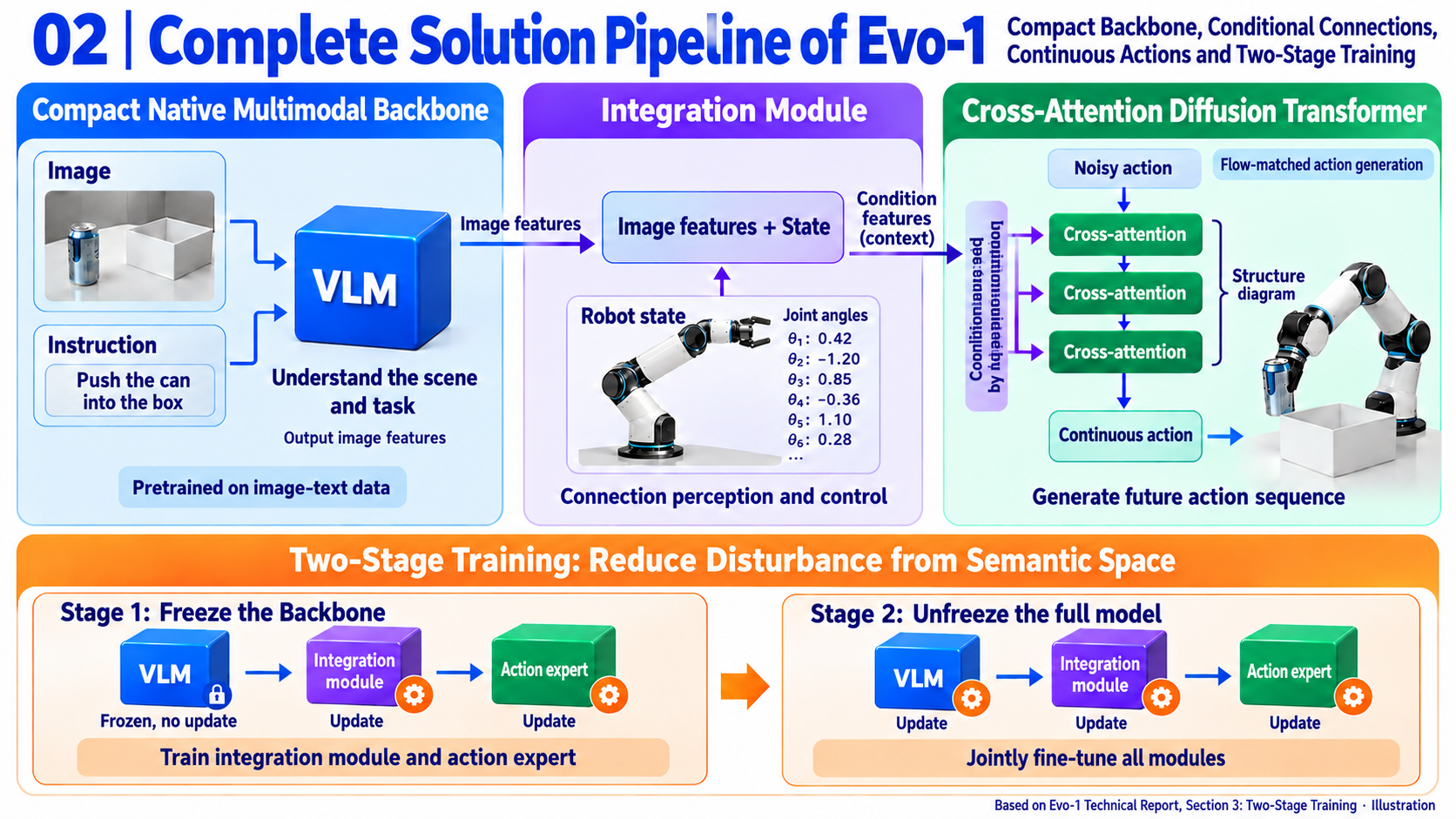
The model encodes what it sees and what it should do, combines this with the robot's current state, and generates future actions from noise.
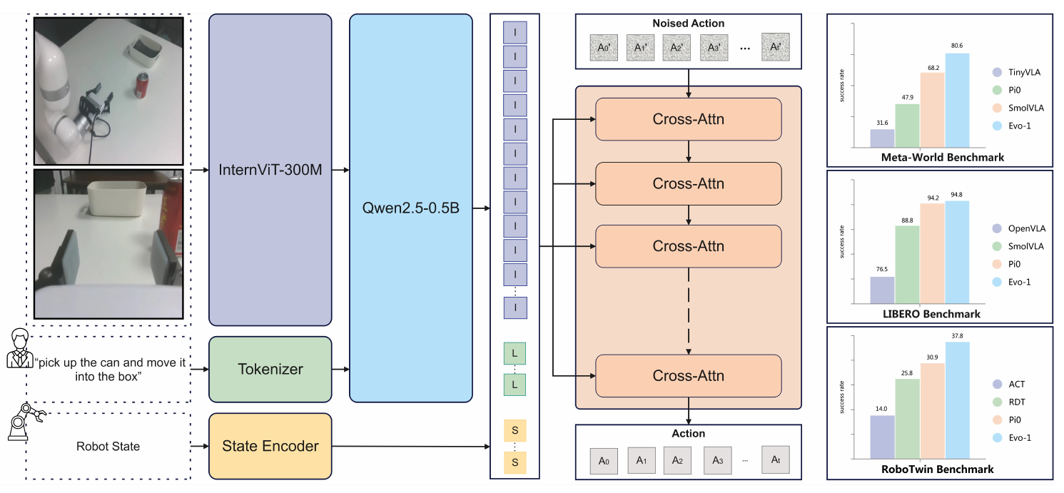
Paper: The three components are the VLM backbone, integration module, and cross-modulated diffusion Transformer. The complete model has 0.77B parameters; do not add the “1B” in the InternVL3-1B name to the total after truncation.
| Path | Raw input | Encoding and processing | Output or role |
|---|---|---|---|
| Vision | N current RGB views | Resize each to 448 × 448 × 3; extract InternViT-300M features; pixel-unshuffle reduces visual token count to one quarter. | Visual embeddings enter the image-text sequence. |
| Language | Natural-language instruction | Tokenize and process with the first 14 layers of the Qwen2.5-0.5B branch. | Fused image-text features at layer 14. |
| State | Robot proprioception | Pad to 24 dimensions by default; Figure 1 includes a state encoder. | Conditioning context for the action expert. |
| Action | Noisy future action chunk | Default shape 50 × 24; processed by an eight-layer Transformer expert. | Same-shaped generation updates and eventually a continuous action chunk. |
N is the camera count and varies by platform; the real xArm6 uses two. Tokens are sequence elements; visual tokens are continuous features, not words. Reducing token count through pixel-unshuffle does not mean shrinking the image width and height each to one quarter.
Paper: InternVL3 jointly learns image-text and text representations during native multimodal pre-training. InternViT-300M is distilled from InternViT-6B. Visual embeddings replace designated <img> placeholders before joint processing with text in a shared decoder. Evo-1 reads layer-14 features and removes subsequent language layers.
Illustrative shapes: One action chunk contains 50 × 24 = 1,200 numbers; a batch of 16 has shape 16 × 50 × 24. The 24-dimensional interface includes padding and does not mean xArm6 has 24 joints. Interpret effective dimensions and units according to each platform's data interface.
Caution: The paper does not fully specify the visual token count, image-text hidden width, action-expert hidden width, or state-encoding details. These implementation boundaries are retained without inferring values from component names. Figure 1's state encoder must not be omitted by claiming that a raw 24D vector is directly added to all image-text features.
Integration: Read the Same Context at Every Layer
Problem: Image-text features describe the scene and task, while state describes the current configuration. Action generation must keep access to these conditions to remain task-directed.
Intuition: Treat multimodal features and state as a shared information source that each action layer reads using its current action representation. The final design is mid-layer cross-attention, Module A in the paper.
In cross-attention, the query Q represents what an action needs to know; keys K match that query, and values V provide the retrieved content. Paper: concatenate layer-14 image-text features and state as K and V, with noisy action representations as Q. All action layers read the same conditioning source.
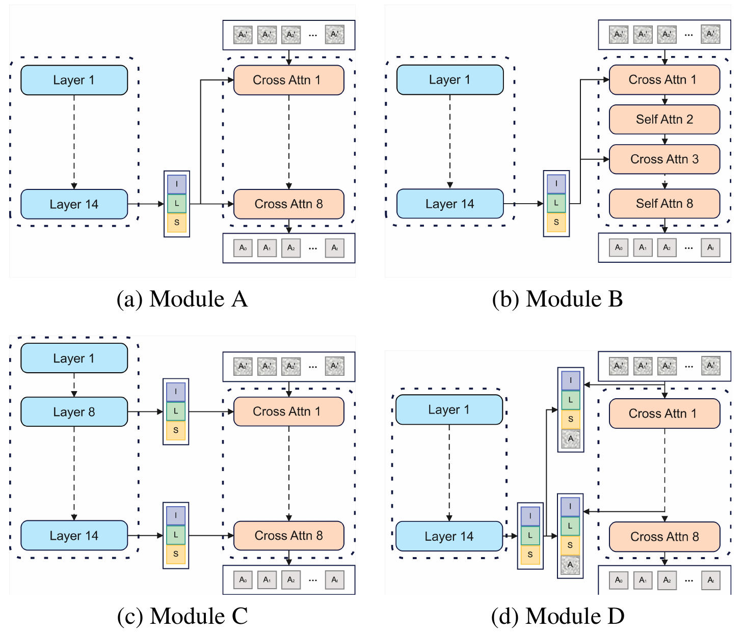
| Design | Connection | Difference from the final design |
|---|---|---|
| A: Mid-layer cross-attention | Layer-14 image-text features and state supply K and V to every action layer. | Chosen design; consistent conditions across layers. |
| B: Mid-layer interleaved cross-/self-attention | Add self-attention after reading conditions. | More interactions within the action sequence. |
| C: Layer-wise cross-attention | Different action layers read VLM features from different depths plus state. | Conditions vary with action-layer depth. |
| D: Joint-KV cross-attention | Image-text, state, and noisy actions all enter K and V. | Actions also become retrieved context. |
Standard attention equation for explanation, not an additional loss proposed by the paper:
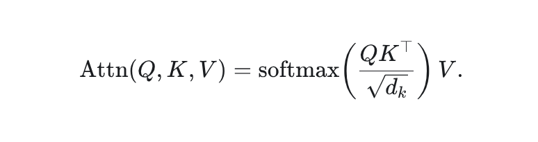
With 50 action positions and M conditioning tokens, one head has Q: 50 × d_k, K: M × d_k, and V: M × d_v; its output is 50 × d_v. d_k and d_v are head widths. Softmax normalizes the M matches for each query. These are explanatory symbols; the paper does not fully report their concrete values.
Minimal example: Suppose one action position assigns weights [0.75, 0.25] to two tokens, whose selected value dimension is [6, 2]. Retrieval gives 0.75 × 6 + 0.25 × 2 = 5. This is an internal feature, not a commanded angle. The next layer can read the context again with its updated action representation.
Caution: The text emphasizes concatenation rather than projection into a shared embedding space, while Figure 1 includes a state encoder. Interpret this as preserving separate conditioning before concatenation, not as evidence that the whole network has no projections or encoders. The exact concatenation axis and encoding widths require implementation details.
Action Expert: Generate a Chunk with Flow Matching
Problem: Image-text features cannot be used directly as joint angles. Future trajectories contain many continuous values that must be generated under the task conditions.
Intuition: Start with a random-noise chunk and learn which direction to move its values toward demonstrated actions. “Diffusion Transformer” (DiT) describes the network architecture; flow matching describes the training objective. The names are compatible.
Equation (3) from the paper:

t is the observation time; A_t is the demonstrated chunk starting then; ε is same-shaped noise; τ is internal generation progress, distinct from robot time. Both arrays default to 50 × 24. The unitless τ is sampled from a Beta distribution and restricted to [0.02, 0.98]; the Beta parameters are not specified.
Minimal example: For one element, take action 0.6, noise −0.2, and τ=0.5; the interpolated value is 0.2. On this linear path, τ=0 is noise and τ=1 is data, although training samples only the truncated interval.
Equation (4), with sampling sources abbreviated:
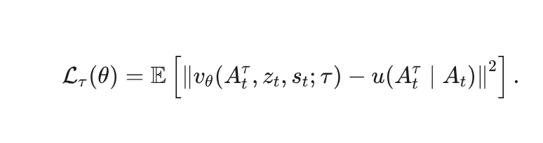
θ denotes trainable parameters; z_t image-text features; and s_t proprioceptive state. v_θ is the predicted time-conditioned velocity field, and u the target generation direction, both with the action chunk's shape. The squared norm compares directional errors across every element, with expectation over demonstration actions and noised samples. The original equation omits the time condition from the network arguments; τ is shown here to match the text's description of a time-conditioned velocity field.
Explanation: Differentiating the linear path in Equation (3) gives A_t−ε; this is an interpretation of the equation, not an explicit expansion of u in the paper. In the example, the target direction is 0.8; predicting 0.7 gives squared error 0.01. The model learns how to move the estimate, rather than directly regressing noisy values to final answers.
Inference repeatedly predicts directions and updates fresh noise under image-text and state conditioning, producing [âₜ, âₜ₊₁, …, âₜ₊₄₉]. The expert uses eight Transformer layers with stacked cross-attention, rather than alternating self-attention.
Illustrative discrete update:
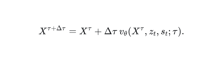
X^τ is the current estimate and Δτ a unitless internal step size. This Euler update explains the velocity field; it is not a fully specified inference algorithm from the paper. Example: a value of 0.2, predicted direction 0.8, and step 0.1 update to 0.28.
Caution: The number of internal updates, numerical solver, and execution schedule are not fully reported. Eight Transformer layers do not mean eight denoising steps, and τ is not robot motion time. Jointly generating a chunk also does not imply independent actions.
Two-Stage Training: Adapt New Modules to Existing Features First
Problem: The backbone already has image-text capabilities, but the action expert is newly initialized. Training everything immediately can let the new modules' gradients distort useful representations toward a limited demonstration set.
Intuition: First teach the action modules to use existing features, then allow joint adaptation. The concrete mechanism is controlling which parameters receive updates.
| Stage | VLM backbone | Integration module and action expert | Purpose |
|---|---|---|---|
| 1: Action-expert alignment | Fully frozen | Trainable | Connect fixed perceptual features to actions. |
| 2: Full-model fine-tuning | Unfrozen and trainable | Continue training | Jointly adapt downstream control from the stage-1 checkpoint. |
Paper: All experiments use distributed training on eight NVIDIA A100 GPUs. Meta-World uses 10,000 steps in stage 1 and 65,000 in stage 2; both use learning rate 1×10⁻⁵, batch size 16, 1,000 warmup steps, gradient clipping 1.0, and weight decay 0.001. Expert dropout defaults to 0.2 and augmentation stays enabled. Other benchmarks use the same two-stage approach with steps adjusted for dataset size (page 11, Tables 4 and 5).
Example: A prediction error updates only new modules in stage 1, but may also change the backbone in stage 2. The stages are not two robot types, nor robot-data pre-training followed by task training.
No explicit semantic-preservation loss is added; the reported action objective is flow matching. Semantic retention relies mainly on initialization and training order, while stage 2 still changes the backbone. The paper does not give wall-clock time or full training cost, so low cost must not be interpreted as completing all training on one consumer GPU.
Training and Inference End to End
Training: demonstration images + instruction → VLM layer-14 image-text features
          demonstrated state → state encoding / integration context
          action chunk + random noise + generation progress → noisy chunk
          context + noisy chunk → action expert → direction prediction → flow-matching loss
          update new modules in stage 1; update the full model in stage 2

Inference: current images + instruction → image-text features
           current state → conditioning context
           fresh noisy chunk → repeated time-conditioned expert updates
           → 50-step continuous prediction → platform control interface → later observations
One-sentence view: A compact backbone interprets scene and goal; integration supplies persistent context; flow matching turns noise into trajectories; two-stage training controls how perception and action adapt.
Experiments: Where the Gains Apply
Simulation: Strong Averages with Uneven Individual Results
| Benchmark and scope | Training and evaluation | Evo-1 average success | Main comparison |
|---|---|---|---|
| Meta-World, 50 tasks | 50 demonstrations per task, 2,500 total; 10 evaluations per task, averaged over five independent runs. | 80.6% | SmolVLA 68.2%; +12.4 percentage points. |
| LIBERO, 40 tasks in four suites | Spatial / Object / Goal / Long; 10 evaluations per task, averaged over five runs. | 94.8% | π0 94.2%; +0.6 percentage points. |
| Four selected RoboTwin 2.0 tasks | 50 demonstrations per task; easy and hard settings; text reports 100 evaluation trials. | 37.8% | π0 30.9%; +6.9 percentage points. |
Source: PDF page 5, Table 1; experimental settings on pages 5–6; supplements on pages 12–13. The distribution of RoboTwin's “100 trials” between difficulty settings is unclear, so no additional total is inferred. This version does not clearly state LIBERO demonstrations per task.
Paper: Meta-World difficulty groups score 89.2%, 76.8%, 77.2%, and 79.2%, each above the listed baselines. LIBERO groups score 92.7%, 97.7%, 96.3%, and 92.3%. Object, Goal, and Long lead, but Spatial is below π0's 96.8%. An average lead does not mean winning every category.
RoboTwin gains are concentrated in Click Alarmclock: 77% / 58% for easy / hard, compared with π0's 63% / 11%. Difficult failures remain: Place Can Basket hard reaches only 1%, below π0's 5%. These results support effectiveness on selected bimanual tasks, not a comprehensive solution to difficult scenes.
Caution: Meta-World and LIBERO baselines come from papers or existing reproductions, and RoboTwin baselines from its official paper; not all methods were retrained uniformly here. Table 1 labels SmolVLA as 2.25B, while efficiency Table 2 uses 0.45B. The discrepancy is not fully explained, so do not treat them as one identical configuration.
Real System: Two RGB Views and Absolute Joint Angles
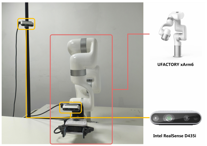
| Item | Paper setting |
|---|---|
| Robot | Six-DoF xArm6 with a parallel gripper, controlled by official xArmAPI. |
| Vision | Fixed environment and wrist RGB cameras; device depth capability is not treated as an input. |
| Recording | LeRobot v2.1 format; synchronized observations recorded at 30 Hz. |
| State and action | Absolute joint angles, consistent with supervision and replay; padded model interface has 24 dimensions. |
| Demonstrations and evaluation | 100 teleoperated demonstrations for each of four tasks, 400 total; 20 trials per task, 80 total. |
Source: page 6 and pages 14–15. Raw camera resolution, demonstration durations, and the complete gripper-field mapping are not explicitly reported. 448 × 448 is the model input size.
Real-World Performance and Inference Efficiency
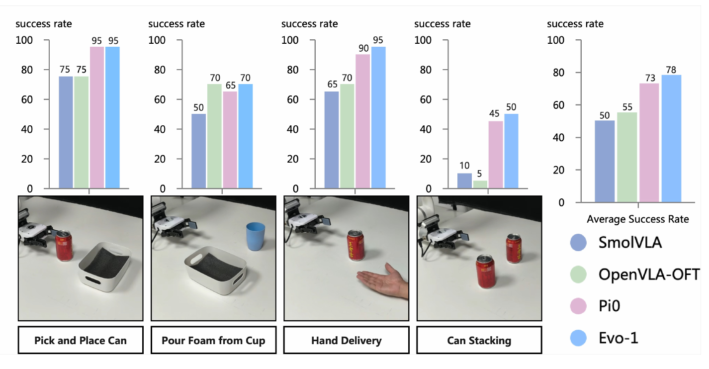
| Task | Paper success criterion | Evo-1 success |
|---|---|---|
| Pick and place a can | Entirely inside the white box, stable, and not rolling out. | 95% |
| Pour foam from a cup | Most foam enters the white box, with visible accumulation and little spillage. | 70% |
| Hand a can to a person | Securely placed in the hand without the person chasing or adjusting to catch it. | 95% |
| Stack cans | Upper can remains stable for at least two seconds without slipping or falling. | 50% |
Source: Figure 4 and success criteria on page 15. The four-task mean is 77.5%, reported as 78%; this is not a 78% score on every task. Stacking remains a weakness.
Table 2: measurements on the specified RTX 4090d GPU.
| Model | Parameters | Average inference VRAM | Average inference rate | Average real-task success |
|---|---|---|---|---|
| SmolVLA | 0.45B | 2.0 GB | 12.7 Hz | 50.0% |
| OpenVLA | 7.0B | 15.1 GB | 7.9 Hz | 55.0% |
| π0 | 3.5B | 17.9 GB | 11.5 Hz | 73.0% |
| Evo-1 | 0.77B | 2.3 GB | 16.4 Hz | 78.0% |
Source: page 7, Table 2. Figure 4 and the results text call one baseline OpenVLA-OFT, while Table 2 calls it OpenVLA. The names are retained without assuming identical implementation settings.
Evo-1 has the fastest inference and highest average success in this comparison, but slightly higher VRAM use than SmolVLA. The 2.3 GB value is average inference memory, not training memory or a guarantee of that rate on any 2.3 GB device.
Caution: 30 Hz is demonstration recording frequency; 16.4 Hz is GPU inference frequency; 50 is the prediction horizon. These describe different stages. Full perception–communication–execution latency is not reported, so 16.4 Hz must not be described as the final robot control rate.
Generalization: Distractors and Position Changes in One Task
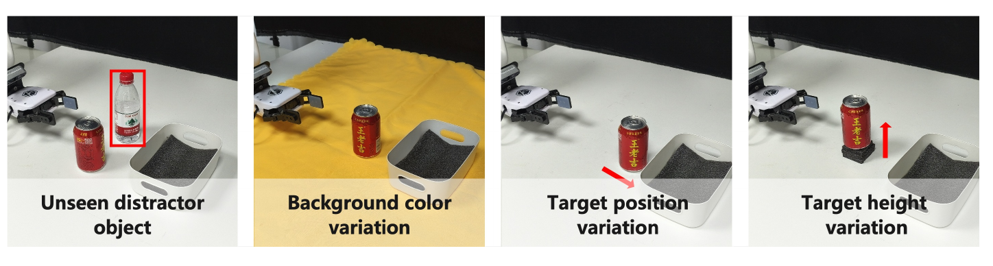
The generalization test uses can-to-box placement with 20 trials per perturbation. The authors define these changes as outside the training distribution.
| Condition | SmolVLA | Evo-1 |
|---|---|---|
| Base scene | 75% | 95% |
| Unseen bottle added | 65% | 80% |
| Yellow tablecloth added | 60% | 75% |
| Target moved back 10 / 20 / 30 mm | 75% / 60% / 60% | 95% / 85% / 80% |
| Target raised 10 / 20 / 30 mm | 75% / 65% / 60% | 100% / 90% / 70% |
Source: page 7, Table 3. Displacement and height are measured in millimeters.
Interpretation: Results support adaptation to these local changes, with Evo-1 above the compared SmolVLA in each condition. Raising the target by 30 mm reduces success to 70%. With 20 trials, a single success changes the score by five percentage points; small differences should not be treated as universal laws. This does not test zero-shot generalization to arbitrary objects, tasks, or robots.
The supplement also shows an SO-100 picking a small block and placing it in a fixed container (pages 15 and 19). Without comparable success, demonstration-count, or efficiency measurements, this is a deployment demonstration rather than quantified proof of adaptation-free cross-robot transfer.
Ablations and Evidence Boundaries
Does Persistent Conditioning Help?
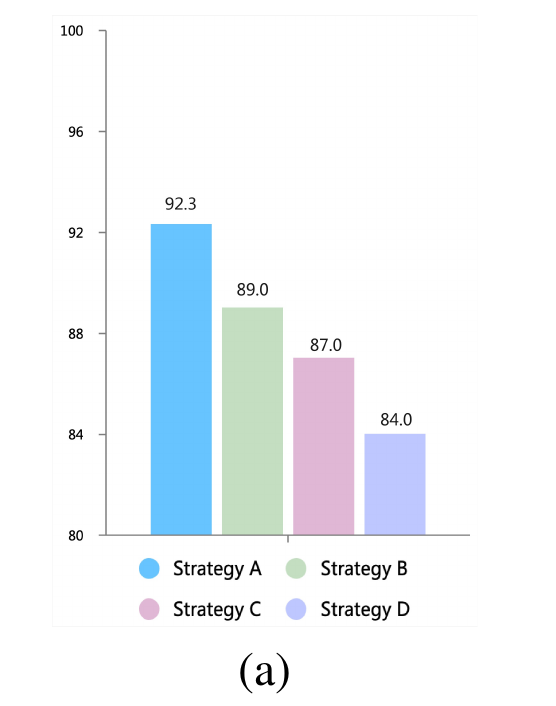
Paper: Modules A, B, C, and D achieve 92.3%, 89.0%, 87.0%, and 84.0%. A exceeds B by 3.3 percentage points and is chosen for the final model.
Interpretation: This supports repeatedly reading the same intermediate image-text features and state. The authors attribute the gain to more continuous conditioning, but the experiment compares four complete designs rather than isolating every factor. It does not show that self-attention is generally harmful or multi-layer feature fusion always inferior.
Does Two-Stage Training Help?
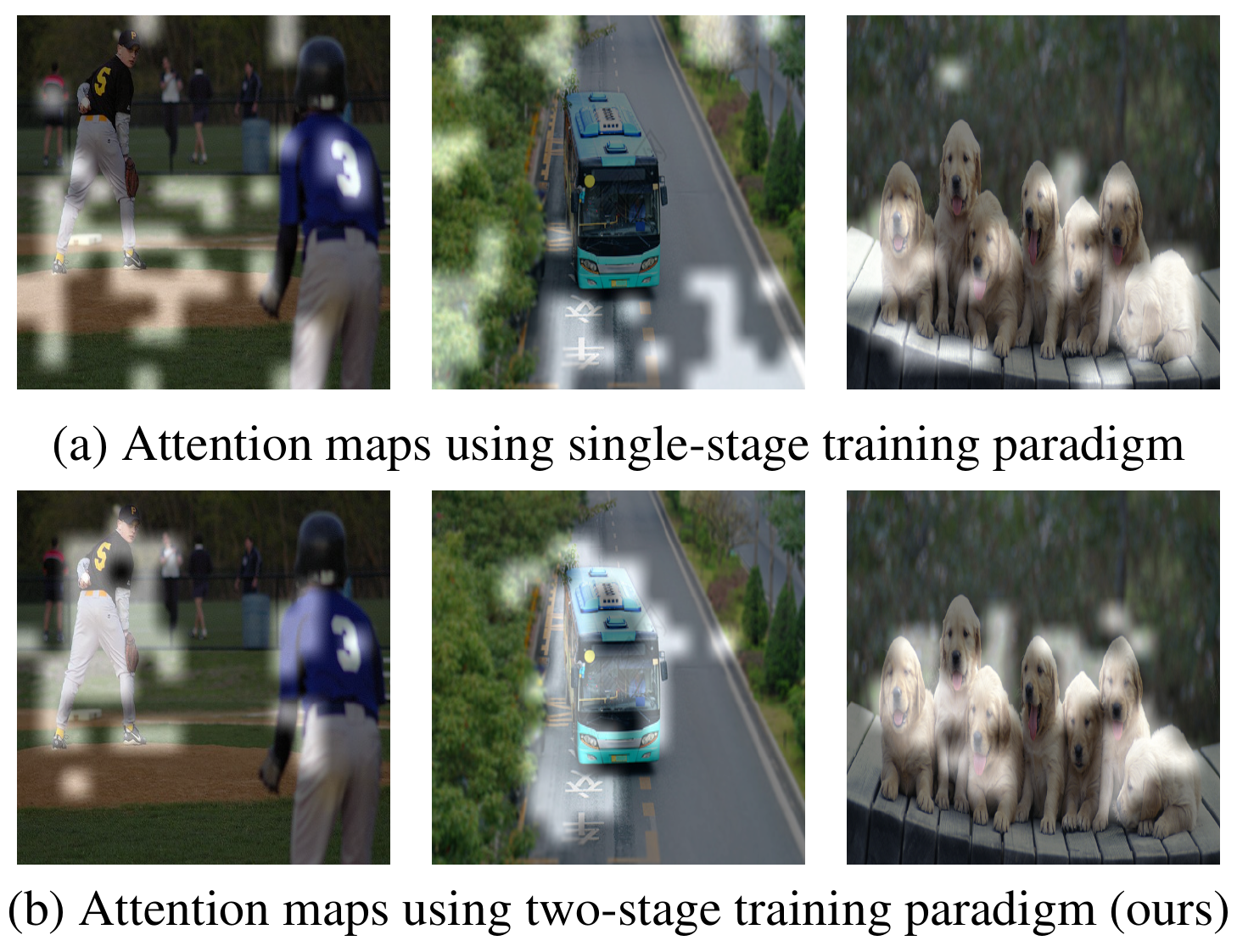
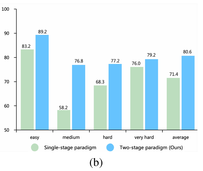
Paper: Two-stage training wins in all four difficulty groups, averaging 80.6% versus 71.4%, a 9.2-point gain. One-stage training updates all modules immediately; two-stage training freezes the backbone first, then fine-tunes jointly.
Interpretation: The controlled success-rate comparison supports the training order. Attention maps suggest clearer image-text focus. Figure 2 also compares Evo-1 and OpenVLA, but different backbones and sizes prevent using that comparison alone to establish the causal effect of two-stage training; the same-architecture ablation is more direct.
Caution: There is no comprehensive quantitative evaluation of general visual question answering, language understanding, or semantic forgetting. Semantic retention has local visualization and task evidence, not proof that all pre-trained knowledge is preserved.
What to Take Away
Evo-1 combines a compact truncated native multimodal backbone, stable cross-attention conditioning, and alignment before joint fine-tuning. This 0.77B combination performs well on the reported simulated and real tasks. The flow-matching action expert still requires target-task demonstrations.
Keep the conclusion within the evidence: RoboTwin covers four selected tasks, real can stacking succeeds 50% of the time, and generalization covers a few changes to one task. Efficiency depends on RTX 4090d measurements, while training uses eight A100s. The paper shows the value of architecture and training design for small VLAs, not universal replacement of larger models or direct deployment on arbitrary robots.