SEEED STUDIO · PAPER DEEP-DIVE

LingBot-VA: A Causal World Model from Future Images to Robot Actions

Causal World Modeling for Robot Control

• Video-action generation
• Causal history
• Real feedback
• Asynchronous correction

arXivRead the paper↗

Hugging Face · LeRobot LingBot-VA Documentation ↗

Key LeRobot Commands

These integration argument fragments accompany the environment, dataset, and output settings for lerobot-eval or lerobot-train, respectively.

• --policy.path=lerobot/lingbot_va_libero_long --eval.batch_size=1: Load the LIBERO-Long checkpoint; current streaming inference maintains a cache for a single environment.
• --policy.attn_mode=flex --policy.use_peft=true: Use block-causal attention and PEFT adaptation during training. The memory needed for AdamW training of the full 5B model cannot be inferred from single-GPU inference requirements.
• --policy.save_predicted_video=true: Additionally decode and save the model's imagined video during evaluation. These predictions and recordings of the actual environment are separate outputs.

A robot needs to open a delivery box. Its camera sees the box and a utility knife, but one image alone cannot tell it whether the seal has been cut, whether the blade is extended, or which step to retry after a failure. If a model only outputs the next arm-motion segment, the relationship between visual changes and action consequences must remain implicit within its policy.

LingBot-VA makes this relationship explicit in generation: predict possible upcoming states in a compressed video space, generate actions from them, then update the context with real images after execution. This introduces challenges: imagined images may be inaccurate, video generation takes time, and the robot cannot keep stopping to wait. This guide follows how the future affects actions, how real feedback corrects predictions, and how computation fits around execution.

Prerequisites: Predicting Images and Choosing Actions

A world model learns how the environment changes. When a gripper rises, for example, a box lid may rise with it or stay still if the grasp failed. Here, the world is the manipulation scene visible to the cameras; the term does not imply a complete, accurate physics simulator.

Inverse dynamics infers actions from a state change: if the gripper is currently outside the lid and should grasp it next, how should it move and close? Forward dynamics predicts consequences from the current state and a given action. They answer how to achieve a change and what a particular action will cause, respectively.

A video latent is the representation produced when a video VAE compresses images. Most prediction happens in this representation, without requiring a playable RGB video before every control step. Autoregressive (AR) means later generation depends on existing history. This model generates continuous variables in blocks, with multiple flow-matching updates inside each block, rather than choosing one discrete word at a time as a language model does.

Keep three time scales separate: actual robot execution time, video/action block indices, and the generation time that gradually turns noise into data. An extra denoising update does not automatically execute another robot action.

Abstract: Paraphrase and Reading Notes

Paraphrase: The authors argue that video world modeling can provide a foundation for robot learning alongside vision-language pretraining. LingBot-VA is an autoregressive diffusion framework that jointly learns future-frame prediction and policy execution. Its three main designs integrate visual and action tokens in a shared latent space through a Mixture-of-Transformers, continually update closed-loop rollouts with real observations, and coordinate action prediction asynchronously with robot execution. Simulation and hardware experiments examine long-horizon manipulation, post-training data efficiency, and generalization to new configurations. Code and models are released.

Reading note: The first design concerns information exchange, the second concerns contact with the real environment, and the third concerns generation latency in the control loop. All three must work together: better image prediction need not mean better actions, stored history does not guarantee disturbance handling, and asynchronous operation does not justify using stale predictions indefinitely. The following sections assess these claims through mechanisms and experiments.

Introduction and Related Work: Bringing Video Generation into Control

The first introduction paragraph identifies a learning burden: when actions are predicted directly from observations, scene semantics, physical changes, and motor control are linked mainly through the same demonstration supervision. The authors call this representation entanglement and suggest that explicitly learning environmental evolution may improve sample efficiency and generalization. The issue is whether dynamics supervision explicitly enters the objective; VLAs with observation history can also use temporal information.

The argument then turns to existing world models. Interactive neural simulators predict action consequences, joint video-action diffusion uses both kinds of supervision, and approaches that first generate target images provide visual goals to a policy. However, long predictions without subsequent real feedback drift away from execution, while blocks without persistent context can lose earlier manipulation state. The authors therefore predict block by block from history and incorporate real observations through a cache.

Section 5 divides related work into vision-language policies and robot world models. The latter may predict low-dimensional latent states, 3D point clouds, or 2D images. LingBot-VA follows video generation, with computation in VAE latent space. Its contribution goes beyond an auxiliary video loss: predicted future representations participate in action generation at inference time.

Here, causal primarily describes temporal dependencies and attention visibility. It organizes generation around available information; it does not establish real-world causality through interventions or guarantee physical correctness. Section 3.2 explicitly allows bidirectional attention within a generation block. The causal boundary mainly separates historical and future blocks.

Overall Process: Predict the Future, Then Infer Actions from Change

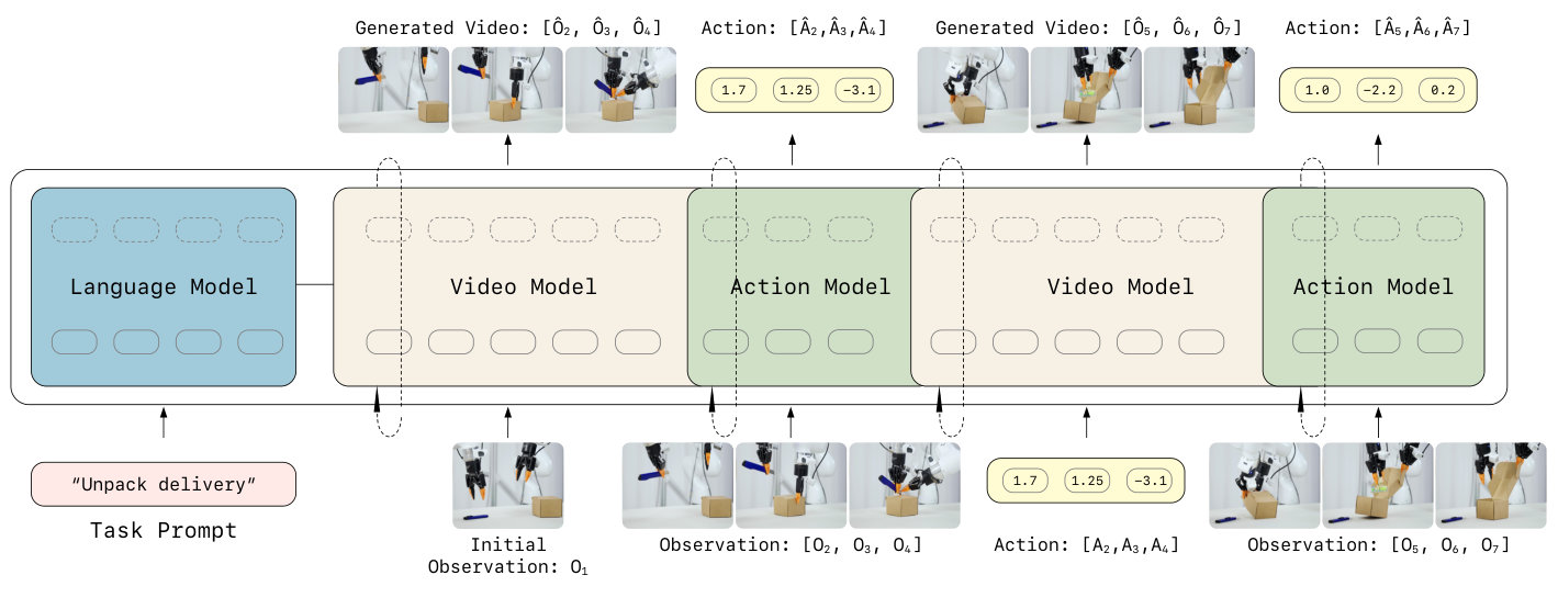
In Figure 2, distinguish the two rows first. The top row contains predicted images and actions; the bottom supplies real observations and executed actions between blocks. Generation on the right reads the updated context, so an imagined open lid does not automatically become a fact in the environment.

Let $o_t$ denote an observation, $z_t=E(o_t\mid o_{<t})$ the latent state from the causal video encoder, $a_t$ an action, and $c$ the language instruction. The conditioning relationships in Section 3.2, Equations (8)–(9), can be organized as:

$$\hat z_{t+1:t+K}\sim p_\theta(\cdot\mid z_{\le t},a_{<t},c), \qquad a_{t:t+K-1}\sim g_\psi(\cdot\mid \hat z_{t+1:t+K},z_{\le t},a_{<t},c).$$

The first expression predicts future latents; the second generates actions conditioned on them. Hats indicate predictions. Following the paper's simplified indexing, each future state corresponds to a control segment; the actual system pairs sparser video with denser actions. Language conditioning, omitted in some shorthand expressions in the paper, is written explicitly here to make clear that instructions are inputs.

For opening a box lid, the current and predicted future representations jointly tell the action branch where the gripper should go and how the lid should change. Past actions and observations also help determine whether it has been grasped. A low-level control interface executes the actions, and the real outcome is encoded back into history. This path generates actions directly from predicted states; it does not enumerate candidate trajectories and select one using an explicit cost function.

View full size

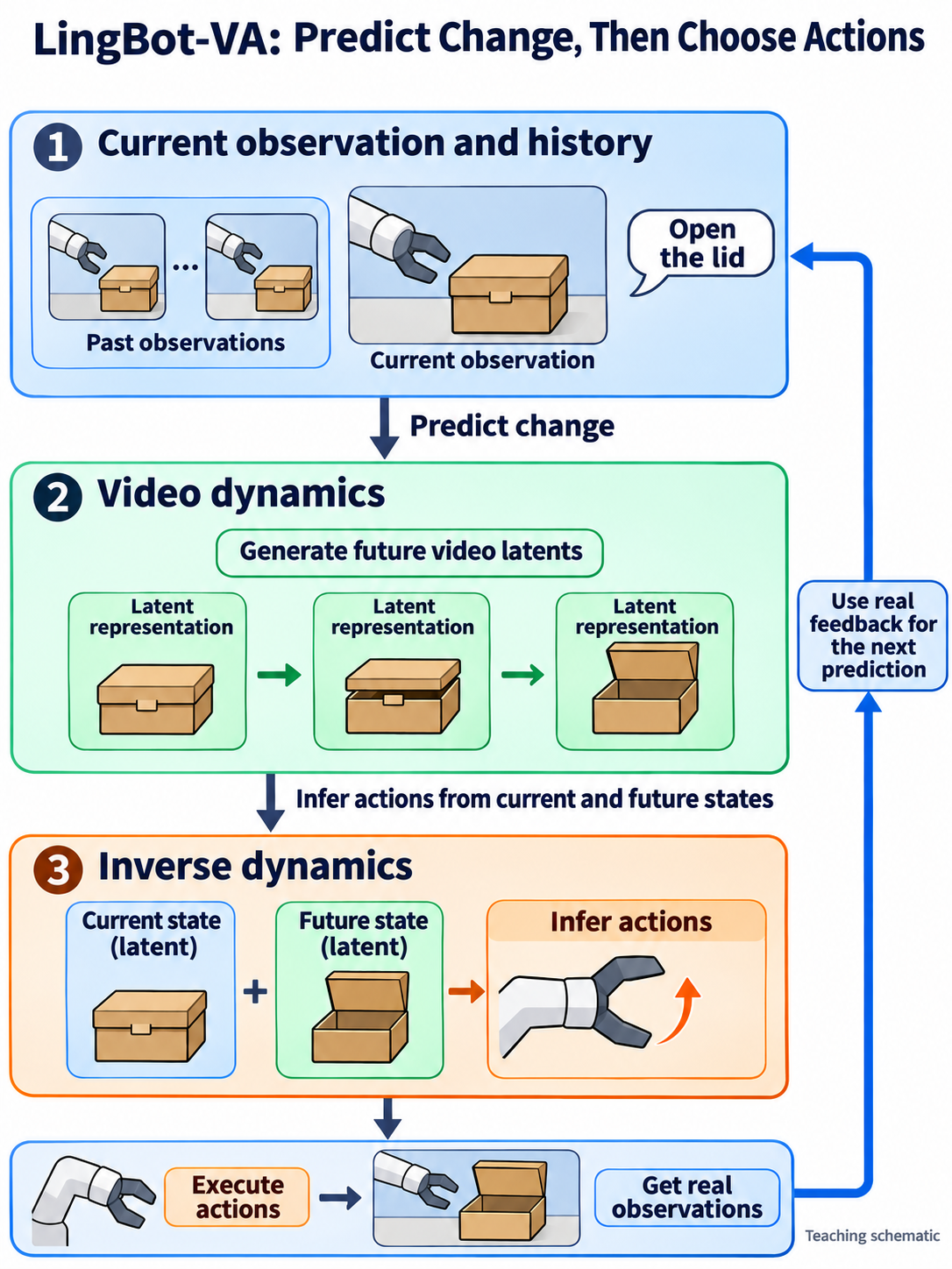
Teaching illustration: green boxes are predicted latent representations; the blue box at the bottom comes from the real camera. Follow the feedback arrow on the right to see how real execution updates the basis for the next prediction.

How Video and Actions Enter One Model

Compress Images while Preserving Different Sampling Rates

The paper uses the Wan2.2 causal VAE to compress video by approximately 4 × 16 × 16 in time, height, and width, then applies spatial 2 × 2 patchification to reduce tokens. Encodings from multiple cameras are concatenated along width. Section 4.2 reports 192 spatial tokens per frame for its configuration. This depends on resolution and camera layout and is not fixed across all LeRobot configurations.

Visual changes are usually slower than changes in control commands. Section 3.3 uses $\tau=4$: each retained video time point is associated with 4 actions. Generating $K=4$ such visual time points therefore corresponds to $4K=16$ action positions. Sparse video sampling and VAE temporal compression are separate operations; they do not jointly mean that the robot only needs to look every 16 steps.

Shape example: With LeRobot defaults frame_chunk_size=4, action_per_frame=4, and action_dim=30, internal action-stream noise can have shape [1,30,4,4,1]: 16 temporal positions with 30 channels each. Valid action channels are selected from the output and converted to [batch,action_steps,robot_action_dimensions]. This is an interface example from the pinned implementation, rather than a universal tensor shape for every platform in the paper.

View full size

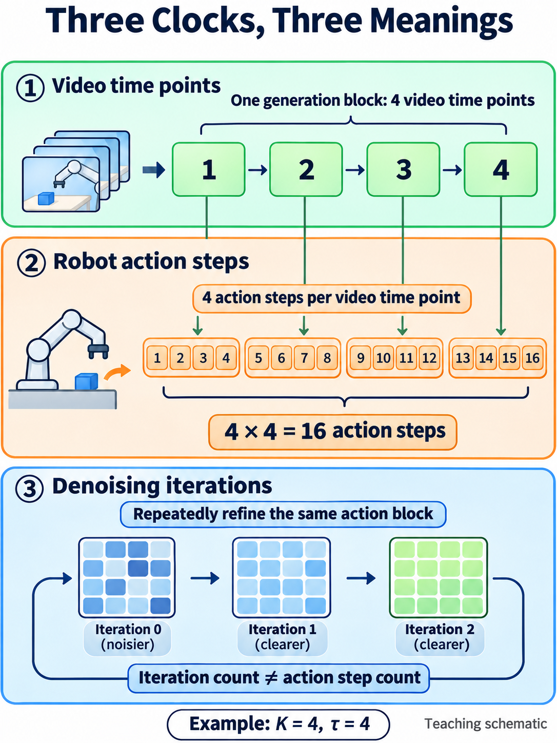
Teaching illustration: the top two rows follow robot time; the bottom row follows generation progress. Each denoising update modifies the same action chunk without adding an execution time point.

MoT: Separate Processing with Attention-Based Exchange

The paper's Mixture-of-Transformers (MoT) has two parameterized branches. The video branch starts from Wan2.2-5B, with hidden width 3072 and 30 layers. The action branch has the same depth but width 768, adding approximately 350M parameters for a total of about 5.3B. High-dimensional visual changes receive more capacity, while low-dimensional control uses a smaller action branch (Section 4.2).

In each layer, video and actions form queries, keys, and values through their own projections. Action features are then projected into a space for joint attention, exchange information with visual features, and return to the action branch. A final linear head maps them back to control vectors. A frozen T5 encoder supplies text conditioning through cross-attention.

MoT addresses how modalities retain their own processing while sharing information. LingBot-VLA 2.0's MoE instead lets tokens select a few feed-forward experts to distribute capacity and active computation. The names are similar, but the mechanisms differ.

The authors also interpolate video weights to the action width and scale initialization by $\alpha=\sqrt{d_v/d_a}$. Substituting 3072/768=4 gives $\alpha=2$. This stabilizes early output distributions across branches of different widths. Figure 7 compares training loss, gradient norms, and validation loss, supporting greater stability than random initialization; these curves are not robot success rates.

The Released Architecture and the Paper's Architecture

The released checkpoint uses a shared backbone, also integrated into LeRobot. It treats video and actions as two generation streams, with separate input/output mappings but shared main Transformer blocks. The paper's asymmetric 3072/768 branches and approximately 5.3B total describe a different parameter organization and cannot directly estimate the shared-backbone checkpoint's size or computation.

Training: Two Flow-Matching Objectives and History Supervision

From Noise to Video and from Noise to Actions

Following the time direction in Section 2, let $z$ be clean video latents and $a$ action data, with independent Gaussian noise $\epsilon_z,\epsilon_a$ of the corresponding shapes:

$$z^{(s)}=(1-s)\epsilon_z+sz,\qquad a^{(s)}=(1-s)\epsilon_a+sa,\qquad s\in[0,1].$$

The networks learn velocity targets $z-\epsilon_z$ and $a-\epsilon_a$, respectively. Section 3.3, Equations (11)–(12), defines $\mathcal L_{\rm dyn}$ through video-latent generation error and $\mathcal L_{\rm inv}$ through action-generation error conditioned on current and future visual representations. The total objective is:

$$\mathcal L=\mathcal L_{\rm dyn}+\lambda\mathcal L_{\rm inv}.$$

Pretraining uses $\lambda=1$. Both terms are squared velocity-field errors, rather than a direct sum of pixel and joint errors. LeRobot additionally weights by noise time and reduces action error using a valid-channel mask, so numerical loss values cannot be inferred from this coefficient alone.

Teaching calculation: Simplify a latent to one number, with data value 0.2 and noise 1.0. At $s=0.5$, the input is 0.6 and the target velocity is 0.2−1.0=−0.8. With an accurate model, an Euler update of $\Delta s=0.1$ gives 0.6+0.1×(−0.8)=0.52; integrating to 1 reaches 0.2. The action stream learns its own direction under its conditioning and noise. Here, $s$ is generation progress, not elapsed robot execution time.

Teacher Forcing: Which History Is Visible during Training?

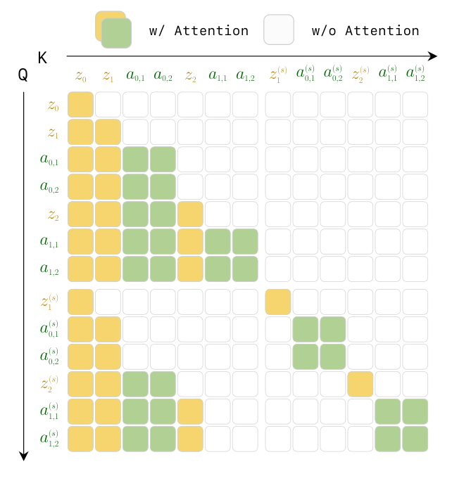
Teacher forcing conditions training on real history from the data, rather than first rolling out a complete model-predicted trajectory. In Figure 3, rows are querying tokens and columns are readable keys. Yellow denotes vision, green actions, and blank entries blocked access. The upper half organizes the history cache; the lower half organizes noisy targets. This is not a simple lower-triangular mask that restricts every token individually: action generation must read the corresponding future visual conditions, and joint generation within a block is allowed.

Real future actions should not directly condition the current prediction. Boundaries between historical and prediction blocks allow training to process multiple time points in parallel in one forward pass. During execution, real camera feedback reenters history, making some training conditions resemble deployment. Predicted future latents, control errors, and feedback latency can still cause distribution shift.

View full size

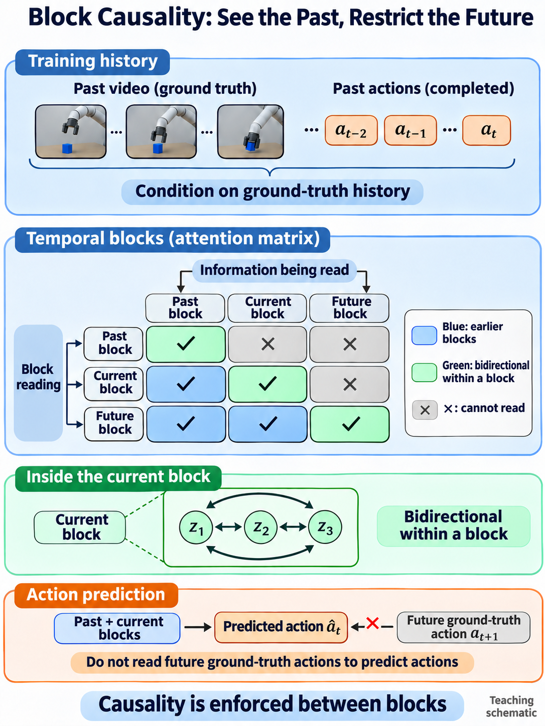
Teaching illustration: read rows to identify who is reading, then columns to identify what is read. This matrix only summarizes temporal-block relationships. Figure 3 in the paper defines detailed visibility between video and action streams, particularly the inverse-dynamics connections to corresponding future visual conditions.

Noisy History: Generate Actions before Video Is Fully Denoised

Equation (10) adds noise to video history with probability 0.5: $\tilde z=(1-s_{\rm aug})\epsilon+s_{\rm aug}z$, with $s_{\rm aug}$ sampled from [0.5,1]; otherwise history stays clean. The action stream thus learns to infer actions from visual representations that remain noisy but contain task structure.

This supports partial video denoising at inference, reserving computation for actions. Algorithm 1 illustrates integration to 0.5; Section 4.2 actually reports 3 video steps to 0.6 and 10 action steps to 1.0. These are a conceptual algorithm and an experimental setting, respectively. Current LeRobot defaults instead use 20 video steps and 50 action steps, with video_exec_step=-1 disabling early truncation. These three settings are not interchangeable, and the paper's 3-step setting cannot estimate the speed of current default code.

Closed-Loop Execution: What to Cache and What to Correct

Update the KV Cache with Real Feedback

A Transformer's KV cache stores the keys and values formed by historical tokens at each layer, avoiding recomputation of the entire history. Algorithm 1 starts with an initial observation, predicts future latents and actions, executes the current actions, collects real observations, and adds real latents and executed actions to the cache.

The cache stores internal model features. It makes history available, while effective use of that history still depends on learning. Context is also finite. Current LeRobot uses attn_window=30 and calls reset for a new episode, clearing the action queue, Transformer cache, and streaming VAE cache. This is neither unlimited memory nor automatic memory retention across tasks.

Asynchrony Requires More than Starting Two Threads

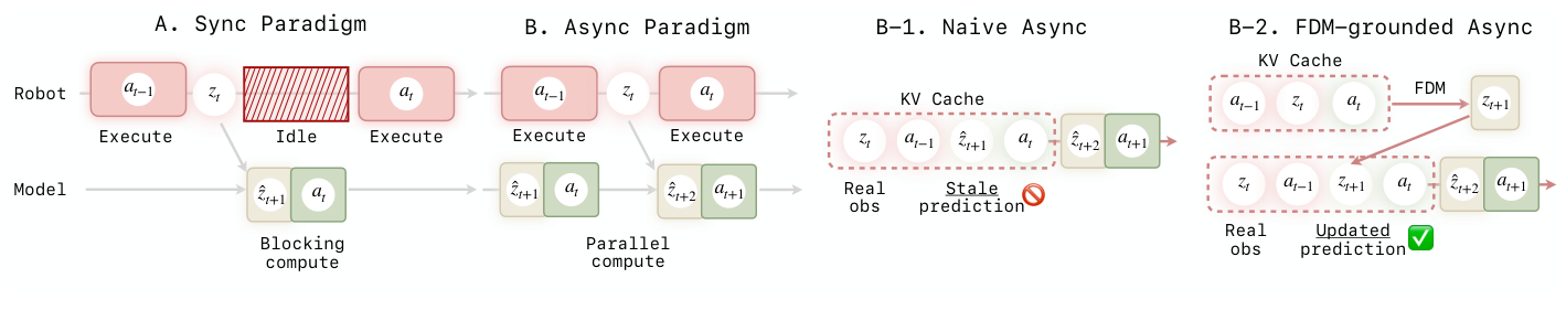
Figure 4A's synchronous sequence is execute, observe, wait for generation, then continue execution. Red hatching marks waiting for computation. Figure 4B predicts the next block while the robot executes the current one, overlapping execution and generation.

The cost is stale information: the current block has not finished when the next is predicted. If the model only reuses imagined images, it may still believe the lid is grasped despite recent real observations showing a slip. Figure 4B-1 illustrates these old predictions continuing to occupy the context.

The paper calls this Forward Dynamics Model (FDM) grounding: a forward-dynamics computation that corrects stale predictions. Starting from the latest real observation and the actions currently being executed, it predicts their outcome again, then uses this realigned future state to predict subsequent video and actions. It uses the model's forward-prediction capability; the paper does not require a wholly separate simulator. Post-training adds the forward-prediction loss in Equation (13), while Algorithm 2 describes coordination between execution and inference branches.

View full size

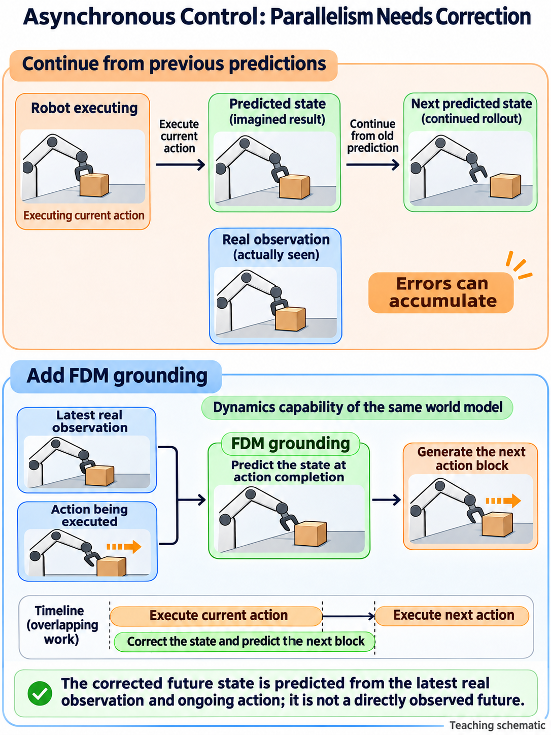
Teaching illustration: the two paths differ in whether the latest feedback is used to predict the current actions' consequences again. The timeline below shows overlapping computation and execution, not direct observation of the future or fixed timing proportions.

Timing example: Suppose executing the current chunk takes 320 ms and generating the next takes 180 ms. A synchronous cycle takes about 320+180=500 ms. If execution fully covers generation, the ideal pipelined cycle is about 320 ms, a speed ratio of 500/320=1.56. This teaching example ignores communication, cold starts, and feedback waiting; it is not a paper measurement. Asynchrony reduces waiting but does not make stale observations current.

Current LeRobot select_action waits until the action queue is empty, updates the cache with buffered real keyframes and the preceding action block, then generates video and actions serially. It implements real feedback between blocks. Algorithm 2 additionally requires parallel execution and prediction, plus FDM grounding of stale predictions.

Data, Action Representation, and Training Stages

Section 4.1 lists six sources—AgiBot, RoboMind, InternData-A1, the OpenVLA subset of OXE, the UMI family excluding DexUMI, and RoboCOIN—plus internally collected trajectories, totaling approximately 16,000 hours of robot manipulation data. Each dataset is split 90%/10% for training and validation. Internet-video knowledge enters mainly through Wan initialization; these 16,000 hours should not be described as entirely action-unlabeled human video.

The canonical action space allocates each arm 7 end-effector-pose dimensions, up to 7 joint dimensions, and 1 gripper dimension: 2×(7+7+1)=30 for two arms. Missing joints are padded. End-effector poses and joint positions are different control representations; the slots do not represent 30 independent physical degrees of freedom.

In the released interfaces, LIBERO uses 7 channels for end-effector deltas and the gripper. RoboTwin uses 16 channels for two arms' XYZ+quaternion+gripper, then converts them into joint trajectories with CuRobo inverse kinematics. Although the 30-dimensional structure reserves joint slots, these two released checkpoints do not directly predict joint positions. Padding alone does not complete adaptation to a custom joint-space dataset.

Stage	Information learned or used	Settings to distinguish
Initialization	Wan2.2 video-generation prior; frozen video VAE and text encoder	The paper's asymmetric branches differ from the current shared-backbone release
Video-action pretraining	Robot video, actions, and language; dynamics and inverse-dynamics objectives	The paper reports 1.4T tokens, peak learning rate 1e-4, BF16, and $\lambda=1$
Downstream post-training	Demonstrations from the target platform and tasks	General adaptation example: 1e-5, 3K steps; six hardware tasks: 50 demonstrations per task, 1e-4, 500 steps
Deployment	Instruction, initial images, subsequent real feedback, and action history	Output actions; video decoding can inspect predictions and need not run at every control step

The method section uses [1,8] to illustrate variable chunk lengths; Section 4.2 reports actual training with [1,4]. Post-training learning rates and step counts also vary by target platform and experiment.

Experiments: Evidence and Conditions

Simulation: Compare within the Same Evaluation

RoboTwin 2.0 training uses 2,500 clean and 25,000 randomized demonstrations across 50 tasks, or 50 and 500 per task. Video is downsampled from 50 Hz to 12.5 Hz while actions remain at 50 Hz. Easy fixes initial configurations; Hard randomizes object poses and scene layouts (Section 4.3.2).

Method	RoboTwin Easy	RoboTwin Hard
π0.5	82.7%	76.8%
Motus	88.7%	87.0%
LingBot-VA	92.93%	91.55%

Table 1 reports mean success across 50 tasks. The margins over Motus are about 4.2/4.6 percentage points, or 8.2/9.1 points in the Horizon=3 group. Here, horizon groups task steps; it is not generation chunk length $K$. Appendix Table S1 also retains weaknesses: Hanging Mug reaches only 40%/28% and Turn Switch 44%/45%, which overall means should not obscure.

Each of the four LIBERO suites contains 10 tasks with 50 demonstrations per task. The paper reports 3 random seeds per suite and 500 evaluations per seed, totaling 1,500 per suite. Table 2 gives:

Method	Spatial	Object	Goal	Long	Average
X-VLA	98.2	98.6	97.8	97.6	98.1
LingBot-VA	98.5 ± 0.3	99.6 ± 0.3	97.2 ± 0.2	98.5 ± 0.5	98.5

Values are success rates in %. LingBot-VA does not exceed X-VLA on Goal. Baseline values come from the X-VLA paper, without fully matched training and implementation conditions. The original ± values are retained; the paper does not specify whether they are standard deviations, standard errors, or confidence intervals. The high success rates apply to these simulation tasks and protocols.

Hardware: Success and Progress Can Tell Different Stories

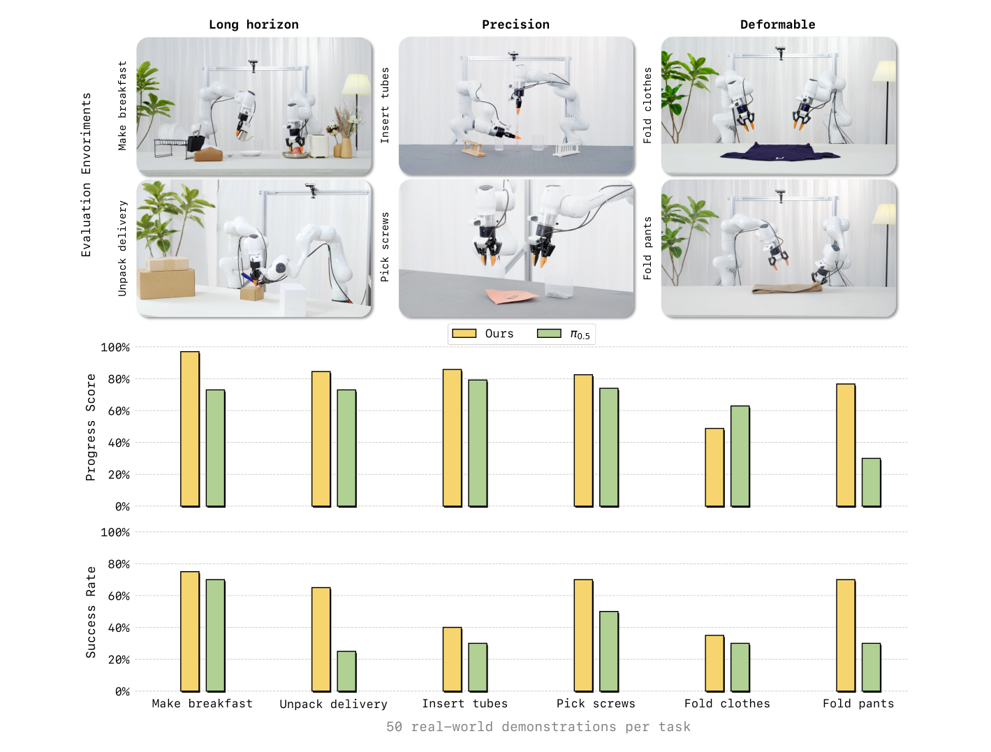
The top of Figure 5 shows six tasks: Make Breakfast, Unpack Delivery, Insert Tubes, Pick Screws, Fold Clothes, and Fold Pants. Each task uses 50 real-robot demonstrations for post-training. Appendix Tables S2–S7 each list 20 evaluations. The progress score is the substep score divided by the maximum score; the success rate is computed from trial Success labels and cannot simply be inferred from whether progress reaches its maximum.

Task	LingBot-VA progress score / success rate	π0.5 progress score / success rate
Make Breakfast	97.0 / 75.0	73.0 / 70.0
Unpack Delivery	84.5 / 65.0	73.0 / 25.0
Insert Tubes	85.8 / 40.0	79.2 / 30.0
Pick Screws	82.5 / 70.0	74.0 / 50.0
Fold Clothes	48.8 / 35.0	62.9 / 30.0
Fold Pants	76.7 / 70.0	30.0 / 30.0

All values are percentages, taken from the appendix tables. Breakfast success is 15/20=75%: even with 97% average progress, one quarter of trials lack a success label. Clothes folding has one more successful trial but a 14.1-point lower mean progress score. This differs from the main text's broad claim of leading on both metrics for all six tasks; Figure 5 itself shows the counterexample.

The table yields mean success rates of approximately 59.2% and 39.2%, but one hardware trial corresponds to 5 percentage points. Results support overall improvement on this task set, without isolating each component's causal contribution. Nor do 50 target-task demonstrations mean the model was trained from scratch on only 50 samples.

Asynchrony and Pretraining Ablations: Benefits with Costs

Table 3 reports the following on RoboTwin Easy:

Setting	Mean success across all tasks	Horizon=3
LingBot-VA reference row	92.9%	93.2%
Asynchronous with FDM grounding	90.4%	85.6%
Naive asynchronous	74.3%	32.9%
Post-training from WAN initialization	80.6%	67.6%

FDM grounding improves over naive asynchrony by 16.1 percentage points overall and 52.7 in the long-task group, supporting realignment of stale predictions with feedback. It still trails the reference row by 2.5 points overall and 7.6 on long tasks. The authors report roughly 2× speed for asynchronous execution, but the table lists neither timings nor test hardware. Success rates show a performance cost to reducing waiting. The speed result also does not directly apply to current LeRobot's serial generation path.

The difference between WAN initialization and full pretraining supports the value of robot video-action pretraining. This comparison changes pretraining experience, so the full gap cannot be attributed to one attention module. Table 3 does not directly compare AR and bidirectional world modeling and therefore does not separately quantify the autoregressive structure's benefit.

What Few-Shot, Memory, and Generalization Tests Show

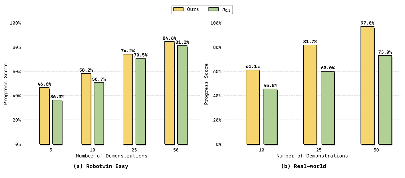
Figure 8 plots target-task demonstration count against progress score. For breakfast on the right, 10 demonstrations yield 61.1% versus 45.5%, a 15.6-point gap; 50 yield 97.0% versus 73.0%. For RoboTwin Easy on the left, 10 demonstrations yield 58.2% versus 50.7%, a 7.5-point gap. The text states 10.3, but the figure associates 46.6−36.3=10.3 with 5 demonstrations. This guide follows the figure's correspondence. These results indicate fewer demonstrations needed under the tested post-training conditions, not lower pretraining data or compute costs.

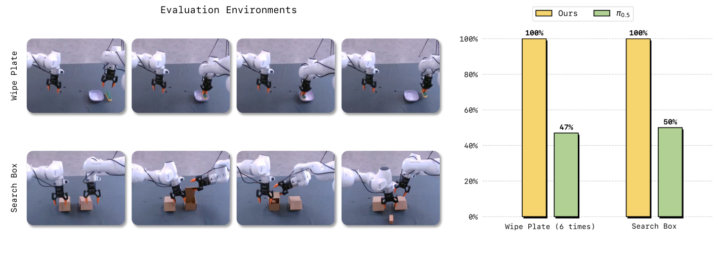
Plate wiping requires exactly six repetitions; box search requires remembering that the right box was empty and then searching the left. Figure 9's right-hand bars report 100% for LingBot-VA on both, versus 47% and 50% for π0.5. These probe temporal-state use more directly than single-frame grasping. However, the paper gives no trial counts for these bars and does not independently remove the KV cache here, so they do not establish reliability on arbitrary long-history tasks.

Figure 10 visualizes object replacements and broader object-position ranges, suggesting generalization. Without a complete out-of-distribution success table or sample counts, a few successful demonstrations cannot establish general robustness. Visual continuity, task completion, and physical correctness remain different levels of evaluation.

LeRobot Integration: Connecting Mechanisms to the Current Interface

LeRobot provides a base model and post-trained LIBERO-Long and RoboTwin checkpoints. Checkpoints store the main trainable Transformer's weights; the frozen VAE, text encoder, and tokenizer are fetched separately during loading, so practical loading also requires these components.

Camera order is part of the input definition. LIBERO places the external view before the wrist view, concatenating latents along width. RoboTwin uses head, left-wrist, and right-wrist views in the robotwin_tshape layout. Swapping camera names without adjusting layout changes spatial meaning. Valid action channels, end-effector-pose conventions, and normalization statistics must also match the checkpoint.

The default 4×4=16 describes an ordinary action chunk. In the pinned code, the first chunk includes the initial conditioning frame and discards its corresponding actions, so it returns (4−1)×4=12 steps; later chunks return 16. The current interface predicts again after the queue empties. Its 20/50 generation updates should not be called control frequencies.

Training forward encodes camera time windows and computes both video and action flow-matching losses. attn_mode=flex is required for the block-causal training path. save_predicted_video adds VAE decoding to inspect predicted environmental changes; evaluation should compare that imagined video with actual execution recordings.

Conclusion

LingBot-VA's central insight is that future representations can condition action generation, but must continually be corrected by the real environment. The video branch learns changes, the action branch infers control from them, and the history cache preserves interaction context. Partial denoising and asynchronous execution address the time cost of bringing generation into control.

Experiments support this approach in the tested simulation, hardware, and few-shot settings while retaining clear limits: lower clothes-folding progress, substantial degradation with naive asynchrony, and a success-rate cost even with FDM grounding. The released shared backbone and LeRobot interface also differ from the paper's full system. These conditions help determine suitable follow-up experiments more than an average success rate alone does.