SEEED STUDIO · PAPER DEEP-DIVE

LBM and MultiTask DiT: How Multitask Pretraining Helps Robots Learn

A Careful Examination of Large Behavior Models for Multitask Dexterous Manipulation

• Diffusion Transformer
• Multitask pretraining
• Data efficiency
• Rigorous evaluation

arXivRead the paper↗

Hugging Face · LeRobot MultiTask DiT Documentation ↗

Key LeRobot Commands

These are LeRobot main argument fragments for lerobot-train, used alongside dataset, output-directory and other settings. See the documentation above for installation requirements.

• --policy.type=multi_task_dit: Select LeRobot MultiTask DiT, an implementation inspired by LBM rather than an exact reproduction of the paper’s system.
• --policy.horizon=32 --policy.n_action_steps=24: Set a 32-step prediction window including history-aligned positions, and execute a 24-step slice; see the article for their distinction.
• --policy.objective=diffusion: Use the diffusion objective; flow_matching is an alternative requiring its own integration settings.

Can demonstrations from multiple tasks help robots learn new tasks with less data and handle environmental changes? This paper holds the policy architecture fixed and uses controlled experiments to measure the benefits of pretraining.

Distinguishing the sources

The TRI LBM paper studies multitask pretraining with a diffusion objective. LeRobot MultiTask DiT is an open-source implementation inspired by this approach and also supports flow matching. The Boston Dynamics Atlas blog describes an application to whole-body control. Their platforms, datasets, and training recipes differ; model sizes, action spaces, and results should be interpreted within each source.

Prerequisites: From Demonstrations to Action Chunks

Training and Inference

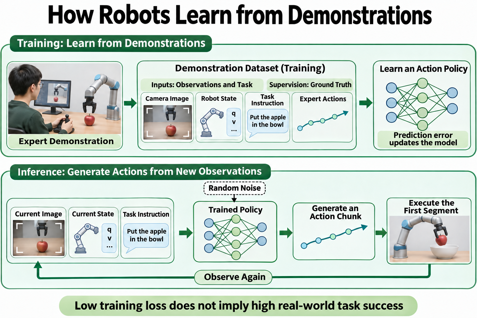
Teaching illustration based on the paper and LeRobot implementation. The example explains the learning workflow.

Behavior cloning uses expert actions as supervision to learn actions conditioned on images, proprioceptive state, and task instructions. Training provides expert future actions; inference generates an action chunk from observations and an instruction.

A Large Behavior Model (LBM) here is a visuomotor policy trained on multitask demonstrations. Image and text encoders from Contrastive Language–Image Pre-training (CLIP) convert images and instructions into conditioning features, allowing task language to guide action generation.

Action Chunks and Generative Models

Action chunking predicts several control steps jointly. After executing a segment, the policy observes again and predicts another chunk. By default, LeRobot generates a new chunk when its action queue is empty, executing the queued segment open-loop. This differs from ACT's overlapping predictions and temporal ensembling. See Action Window and Execution Segment.

A scene may admit several valid trajectories, whose average may be unsuitable. The diffusion generative model learns a conditional distribution over trajectories, generating actions from random noise under observation conditioning.

Diffusion time describes denoising progress, not the robot's physical motion. Below, $t$ denotes physical time and $k$ a discrete denoising step.

Abstract: The Value of Pretraining

Abstract Summary

Imitation learning can solve complex manipulation tasks, but the practical benefits of large robot models remain difficult to evaluate reliably. The authors extend Diffusion Policy to multitask data and compare it with single-task policies using matched random seeds and automated scoring in simulation, and blind testing with randomized policy order in the real world.

Multitask pretraining followed by fine-tuning improves success and robustness while reducing the demonstrations needed for new tasks. Within the evaluated settings, larger and more diverse pretraining datasets generally yield greater benefits.

Commentary

• A fixed core architecture helps separate pretraining benefits from model-size effects.
• The data-efficiency findings concern task-specific fine-tuning, rather than zero-shot learning.
• Initial conditions, trial order, and scoring are controlled, with statistical analysis of the results.

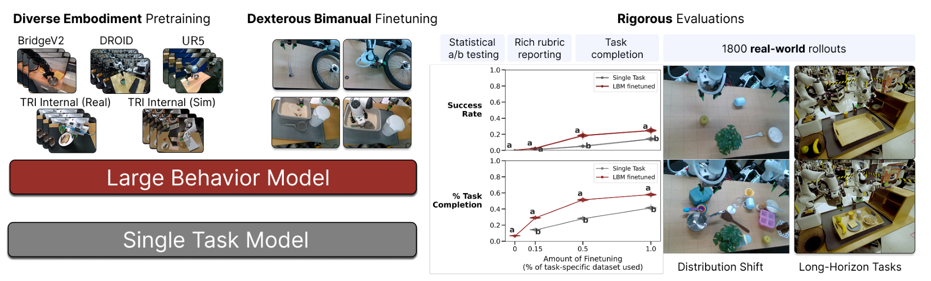
Original Figure 1 (PDF p. 2). Left: pretraining followed by fine-tuning versus single-task training. Right: real-world trials and statistical comparisons.

Introduction and Related Work

The Introduction's Three Paragraphs

Paragraph 1: The gap between hardware capabilities and autonomy motivates learning from demonstrations. Robot hardware supports diverse behaviors, yet reliable autonomy often remains limited to simple tasks or structured environments. Behavior cloning replaces task-specific programming with demonstrations. Its progress in contact-rich manipulation, deformable objects, and bimanual coordination motivates the study of general-purpose manipulation.

Paragraph 2: Brittle single-task policies raise a question about pretraining. Single-task behavior cloning struggles outside its training distribution. LBMs use multitask demonstrations to broaden experience, but how much of their observed success comes from multitask pretraining remains unclear. This question motivates controlled evaluation.

Paragraph 3: The authors establish the experimental scale and state three findings. Models are trained on approximately 1,700 hours of demonstrations and evaluated in simulation and roughly 1,800 controlled real-world trials. The three findings are: fine-tuning requires fewer target-task demonstrations to reach comparable performance; with equal target-task data, fine-tuned models perform better when aggregated across tasks; and these benefits increase when deployment conditions differ from training. The following sections examine the evidence and its scope.

Related Work

Area	Prior work	This paper's focus
Generalist robot policies and VLAs	Extend capabilities through multitask data, pretrained representations, and action generation	Quantify pretraining benefits with a fixed architecture
Large-scale robot datasets	Expand data through teleoperation, public datasets, simulation, and handheld devices	Standardize observations and actions; study data scale and diversity
Robot evaluation	Simulation benchmarks, physical object sets, remote robots, and success metrics	Compare policies using blind trials, randomized order, scene resets, and milestone scoring

The paper does not provide a systematic comparison across VLA architectures or establish that DiT always outperforms VLAs.

Core Method: Conditional Diffusion Transformer

Architecture

Intuition: Images locate objects, instructions specify the task, and proprioception describes the robot's current configuration. The network encodes this context and iteratively refines a noisy action chunk into a trajectory suited to the scene.

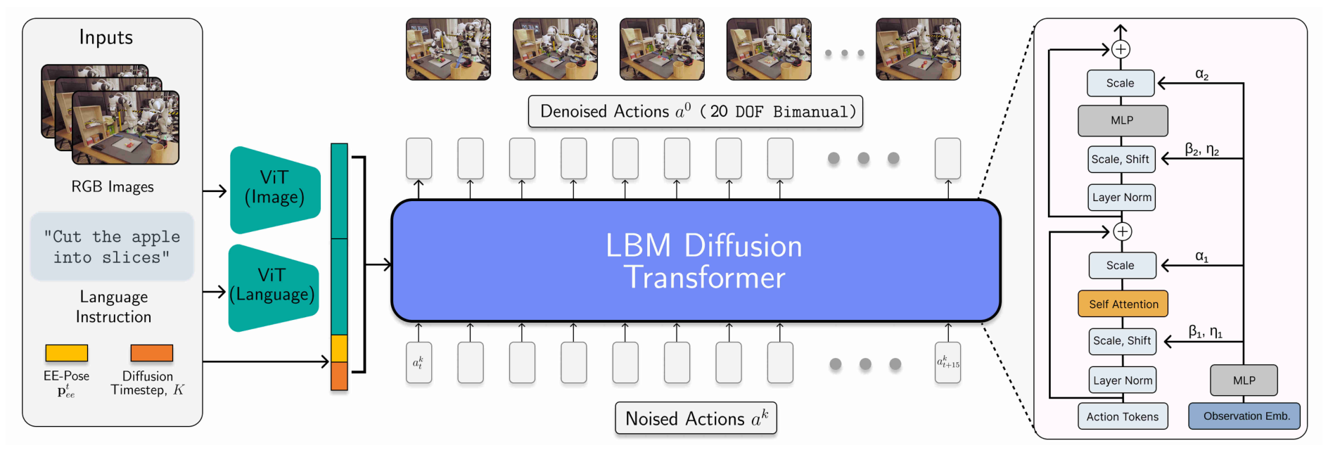
Original Figure 9 (PDF p. 12). Observation encoding on the left, action denoising in the center, and Transformer conditioning modules on the right.

The vision encoder summarizes each image with its classification (CLS) token. Its weights are updated during training and shared across cameras. The text encoder produces a fixed-length instruction representation; its backbone is frozen, while the subsequent projection is trainable. The Diffusion Transformer (DiT) applies self-attention along the action sequence and predicts noise for the entire chunk. Tokens here are feature units and may be continuous vectors.

Observation and Action Dimensions

The paper uses two observation frames with up to six RGB views, zero-padding missing cameras. Proprioception includes end-effector poses relative to the base and to the other end-effector, plus gripper widths, rather than a vector of joint angles.

Action trajectories are represented relative to the current observation (Sections IV-D1 and IV-D2 of the paper). Each hand's action contains three translation components, a six-dimensional rotation representation, and one gripper-width value. The bimanual action dimension is therefore:

$$D_a = 2\times(3+6+1)=20.$$

$D_a$ is the action dimension per control step. The network outputs 16 steps, giving a $16\times20$ sample with 320 values. The 6D rotation representation uses the first two rows of a rotation matrix; it does not denote six rotational joints. These 20-dimensional outputs cannot directly drive a single-arm joint controller.

The paper concatenates 6,732 observation features across the two frames and uses eight DiT blocks with hidden dimension 768. LeRobot computes the conditioning dimension from its camera count, state dimension, and configuration.

Diffusion Training: Predicting Noise

Let $A_t^0\in\mathbb{R}^{H\times D_a}$ be a clean action chunk and $O_t$ the visual, language, and state context. Training samples a noise level $k$ and Gaussian noise $\epsilon$. The standard denoising diffusion probabilistic model (DDPM) formulation below explains the objective: mix actions with noise according to the noise level, then predict the added noise.

$$A_t^k=\sqrt{\bar\alpha_k}A_t^0+ \sqrt{1-\bar\alpha_k}\epsilon,\qquad \mathcal{L}_{\mathrm{diff}}= \mathbb{E}\left[\left\|\epsilon-\epsilon_\theta(O_t,A_t^k,k)\right\|_2^2\right].$$

Here, $H$ is the chunk length, $D_a$ the action dimension, $\bar\alpha_k$ the cumulative signal-retention factor in the noise schedule, and $\epsilon_\theta$ the DiT noise prediction. The expectation covers samples, noise, and denoising levels. Equation (2) in the paper gives the noise-prediction loss and writes noising as $A_t^k=A_t^0+\epsilon_k$. Here, the standard DDPM formulation explains LeRobot's add_noise path; it is not a term-by-term expansion of the paper's expression.

Illustrative example: For a normalized action value of $0.6$, $\bar\alpha_k=0.64$, and noise $-0.2$, the noisy input is $0.8\times0.6+0.6\times(-0.2)=0.36$. The network receives $0.36$ and the observation context; its target is the noise $-0.2$. This scalar example illustrates one element; the model predicts noise for the whole chunk jointly.

How DiT Uses Observation Conditioning

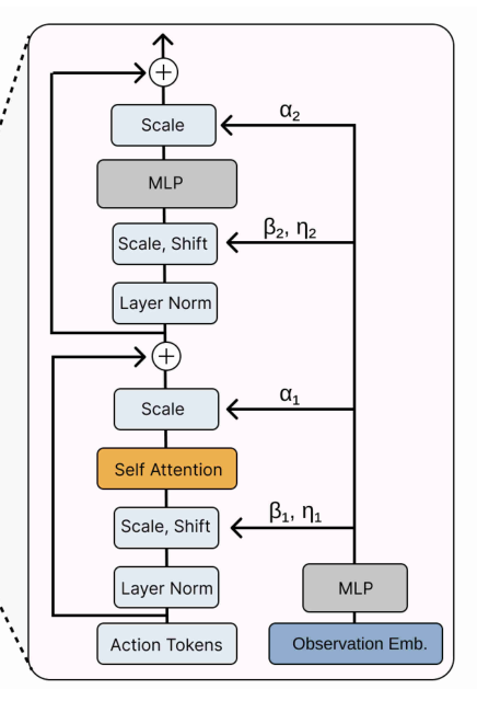
Projected action vectors form a sequence of $H$ tokens. Self-attention connects control steps, while adaptive layer normalization (adaLN) conditions action features by generating feature-wise scales and shifts from the scene and task. This modulation can be written as:

$$\operatorname{Mod}(x,c)= \left(1+s(c)\right)\odot\operatorname{LN}(x)+b(c).$$

$x$ denotes hidden action features; $c$ combines vision, text, state, and denoising-step conditioning. $\operatorname{LN}$ is layer normalization, $s(c)$ and $b(c)$ are the predicted scale adjustment and shift, and $\odot$ denotes element-wise multiplication. These parameters are broadcast across the action sequence, while attention models relationships between actions. LeRobot also predicts gates for the attention and multilayer perceptron (MLP) residual branches.

Illustrative example: A normalized feature of $0.5$, scale adjustment of $0.2$, and shift of $0.1$ produce $1.2\times0.5+0.1=0.7$. Different conditions can yield different scales and shifts. These are internal feature parameters, rather than commands sent directly to the robot.

Architecture: Encoded observations are concatenated into a fixed-length conditioning vector that modulates action features through adaLN. The authors' interpretation: Inconsistent performance without fine-tuning may partly reflect weak language guidance from the small language encoder. The paper does not isolate conditioning compression in an ablation, so it does not establish that compression itself limits language capabilities.

Figure 9: Enlarged conditioning module

Detail from the right of original Figure 9 (PDF p. 12). Conditioning embeddings generate scales, shifts, and gates for the attention and MLP branches.

Inference: Denoising and Execution

At inference, the policy encodes current observations and repeatedly applies the same DiT to denoise a random action chunk. The paper uses denoising diffusion implicit model (DDIM) sampling: the trained noise predictor iteratively updates the chunk. After executing a selected prefix, the policy generates another chunk from new observations.

Control frequency, chunk length, and sampling steps are distinct. The paper generates 16 action steps and replans after executing eight. Generating one chunk requires multiple DiT evaluations. The reported 10 Hz policy loop does not imply ten new chunks per second or guarantee latency on other hardware.

Training: Pretraining and Fine-Tuning

Robots and Demonstration Data

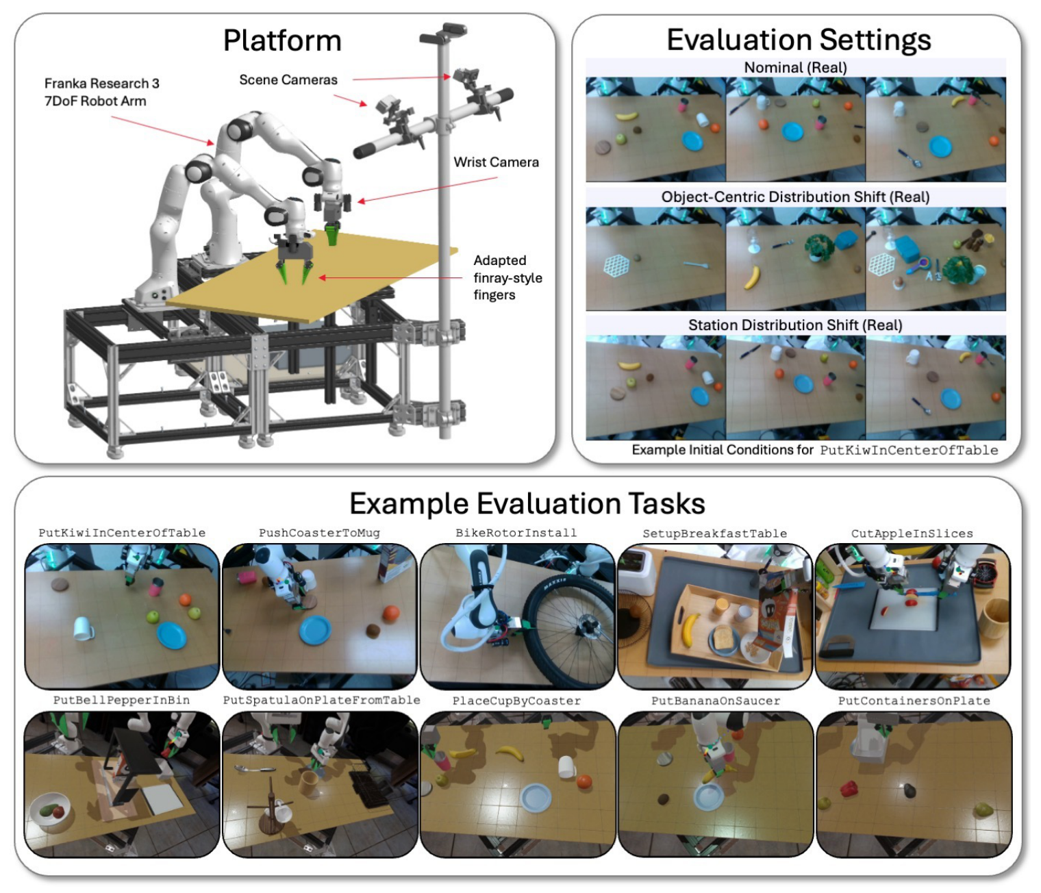
Original Figure 10 (PDF p. 14). Top left: arms and cameras. Top right: environmental changes. Bottom: placement and multistep dexterous manipulation tasks.

The paper uses two Franka FR3 arms with parallel grippers and custom finray-style fingers. The newer platform has two scene cameras and two cameras per wrist, providing six RGB views. Data span hardware generations; real-world evaluation uses the newer platform. Differential inverse kinematics and joint impedance control track end-effector targets, with collision avoidance handled by the lower-level controller. End-to-end learning still depends on these execution interfaces.

Data source	Reported scale	Role
TRI-Ramen-Real	468 hours; 362 tasks; 46,063 demonstrations	Internal real-world bimanual robot data
TRI-Ramen-Sim	45 hours; 41 tasks; 7,348 demonstrations	Simulation data corresponding to the real platform
TRI-Ramen-UMI	32 hours; 129 tasks; 10,851 demonstrations	Manipulation collected outside the laboratory with handheld devices
OXE-Ramen	Approximately 1,150 hours	Curated, standardized subset of public Open X-Embodiment data

The first three sources total approximately 545 hours, 532 tasks, and 64,262 demonstrations. Including OXE-Ramen gives approximately 1,695 hours. The 532-task count covers only internally collected data.

Data Alignment and Normalization

Data sources require consistent coordinate frames, pose units, gripper widths, and image processing. The paper converts single-arm data to a bimanual format by zero-padding the missing arm and randomly swapping sides. Weighted sampling prevents larger sources from dominating batches.

More distant future actions typically span wider ranges. The paper computes quantiles separately by feature dimension, relative timestep, and data source. It maps the 2nd–98th percentile interval to $[-1,1]$ and clips to $[-1.5,1.5]$; the 6D rotation representation is excluded from this scaling.

LeRobot difference: The pinned version defaults to MIN_MAX for states and actions and MEAN_STD for images. It does not automatically reproduce the paper's source- and timestep-specific quantile normalization. Such preprocessing differences also affect results.

Training Configuration

Stage	Initialization and data	Learning rate	Global batch size	Training steps
Multitask pretraining	Full data mixture; CLIP-pretrained vision and text encoders	3e-4	2,560	48,000
Real-world task fine-tuning	LBM weights plus target-task demonstrations	2e-5	320	30,000
Simulation task fine-tuning	LBM weights plus target-task demonstrations	2e-5	320	10,000
Real-world single-task baseline	No robot multitask pretraining; same CLIP initialization	2e-5	320	100,000
Simulation single-task baseline	Same initialization; target-task demonstrations only	2e-5	320	25,000

The vision encoder uses one tenth of the learning rate of the other trainable components. Training images are resized to 256×342 (height × width), randomly cropped to 224×224, and color-augmented. Inference uses a center crop.

Training “from scratch” means without robot multitask pretraining; CLIP initialization is retained. Single-task baselines receive more target-task training steps.

Evaluation Methodology

Task Splits and Scoring

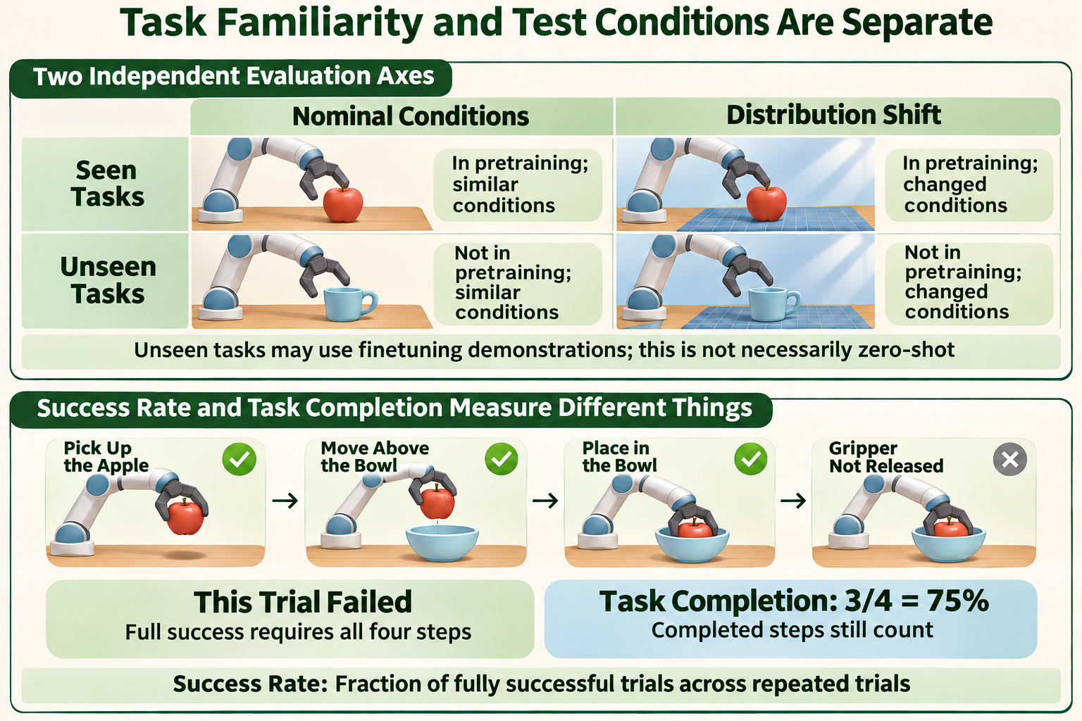
Teaching illustration based on the paper. The four-step apple-placement rubric explains the metrics and is not a record of an evaluated task.

The upper panel separates seen/unseen tasks from distribution shift. Unseen tasks may still provide fine-tuning demonstrations. Distribution shift refers to changes in test conditions, such as distractors, object combinations, or robot stations.

The lower panel uses four milestones to distinguish success rate (SR) from task completion (TC). If the apple reaches the bowl but the gripper has not released it, three of four milestones are complete: TC is 75%, yet the trial is unsuccessful. This is an illustrative scoring example.

$$\mathrm{SR}=\frac{N_{\mathrm{success}}}{N_{\mathrm{trials}}},\qquad \mathrm{TC}_i=\frac{\sum_{j=1}^{M}m_{ij}}{M}.$$

$N_{\mathrm{trials}}$ counts trials and $N_{\mathrm{success}}$ counts fully successful trials. $M$ is the number of milestones; $m_{ij}\in\{0,1\}$ indicates whether trial $i$ completes milestone $j$.

Blinding, Randomization, and Resets

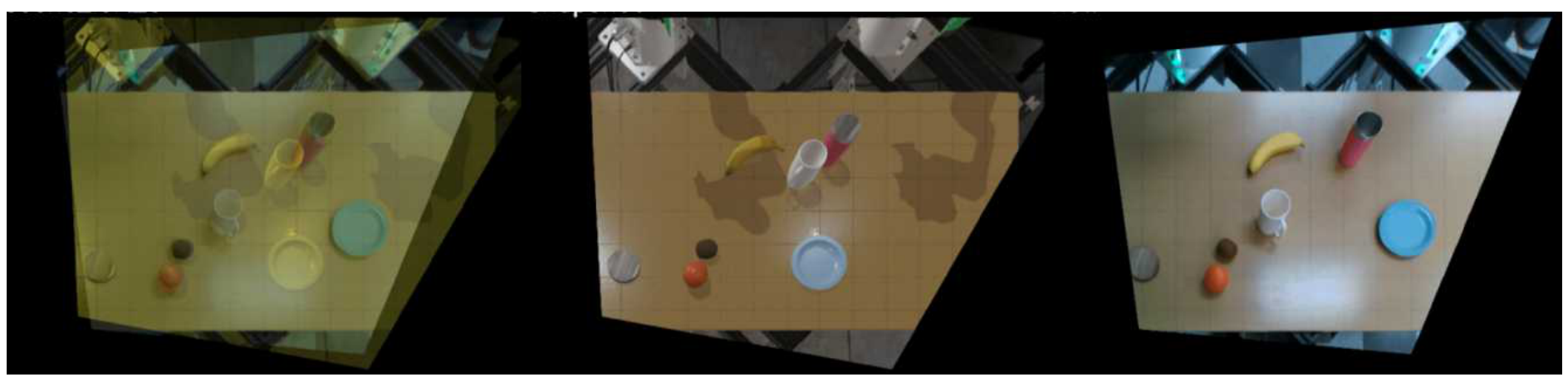
Original Figure 8 (PDF p. 11). Left: an overlay of the target and current scene assists resets. Center: target scene. Right: current scene.

Evaluators are blinded to policy identity. Policies run in randomized order from matched initial conditions, with resets after each rollout to reduce order, lighting, and placement biases. Simulation uses matched random seeds; real-world resets use image overlays. Test initial states do not simply replay individual training demonstrations.

Real-world evaluation includes three seen and five unseen tasks; simulation includes 16 seen and eight unseen tasks. Each task–policy–condition combination is scheduled for 50 real-world or 200 simulation rollouts. A few simulation combinations have fewer than 200 because of missing data. The analysis covers approximately 1,800 real-world and over 47,000 simulation rollouts.

Violin Plots and Statistical Comparisons

SR violins show Bayesian posteriors over the true success probability, estimated from success/failure outcomes. Individual-task TC plots mainly show empirical completion distributions; some aggregate and data-efficiency plots instead show posteriors over mean completion. These represent different quantities.

The paper uses Compact Letter Display (CLD) to summarize statistical comparisons. Groups with no shared letter differ significantly. A shared letter means no significant difference was detected, rather than equivalent performance. Interpret the letters together with the caption, statistical test, and comparison scope.

Results and Limitations

Completion on Unseen Tasks

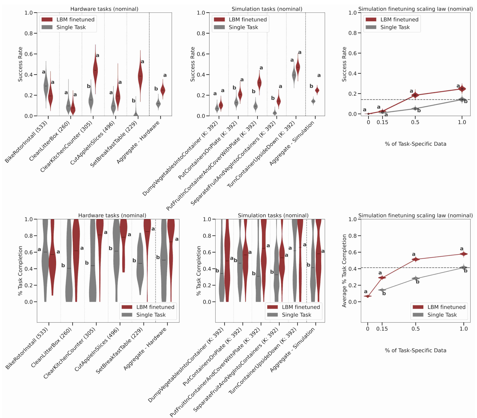
Original Figure 4 (PDF p. 7). Unseen tasks under nominal conditions. Top: SR. Bottom: TC. Columns: real-world tasks, simulation tasks, and simulation data efficiency. Red: pretrained and fine-tuned LBM. Gray: single-task baseline.

Full success remains difficult on complex tasks, but fine-tuned LBMs generally complete more milestones. Among five complex unseen real-world tasks, TC is significantly higher than the single-task baseline on four, while SR is significantly higher on only two.

Aggregate gains are more consistent, but some individual differences are insignificant or favor the baseline. Policies may remain inactive at the start or attempt the wrong task, so individual results and failure cases matter.

Robustness: Do Gains Persist When Test Conditions Change?

Simulation distribution shifts primarily alter appearance: unseen environment lighting maps, different lights and camera parameters, and changed object and table textures or colors. Some scenes also include distractors. The authors compare fine-tuned LBMs with single-task baselines under these changes to test whether pretraining gains persist.

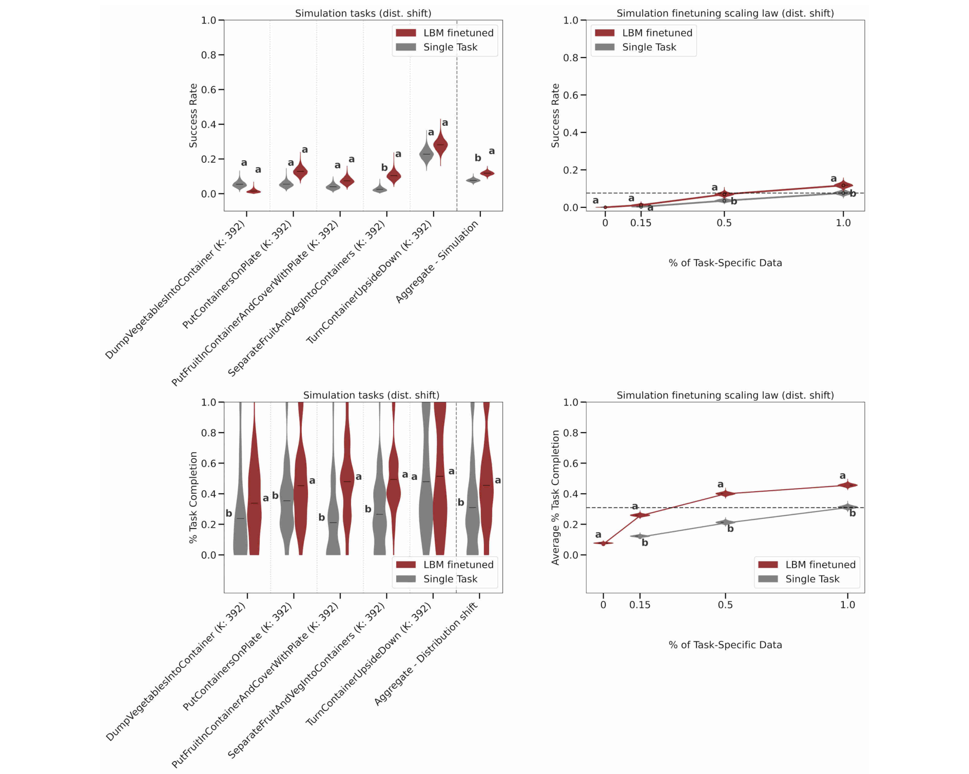
Original Figure 6 (PDF p. 9). Top: SR. Bottom: TC. Left: individual tasks and aggregate results. Right: varying fractions of target-task data. Red: pretrained and fine-tuned LBM. Gray: single-task baseline. Compare with the simulation panels in Figure 4; Figure 6 contains no real-world results.

For five complex unseen simulation tasks under distribution shift, TC is significantly higher than the baseline on four tasks, but SR is significantly higher on only one. On seen simulation tasks, the number with significantly higher SR increases from 3/16 under nominal conditions to 10/16 under distribution shift; the aggregate success-rate gap also widens (Section III-A and Figure 2).

These findings support greater robustness of fine-tuned LBMs under the tested shifts, even though absolute performance declines on most tasks after the changes. Completing more milestones may still leave full success rare. Simulated appearance changes also differ from real-world station and object changes.

Data Efficiency on New Tasks

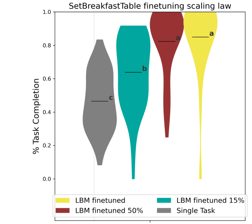
Original Figure 5 (PDF p. 8). Real-world data efficiency: the vertical axis is TC. Each group compares LBMs fine-tuned on different data fractions with a single-task baseline trained on all target-task data.

On the real-world SetBreakfastTable task, an LBM fine-tuned on 15% of target-task data achieves significantly higher TC than the single-task baseline trained on all of it. This result concerns completion, rather than success rate.

Interpolation of aggregate curves for complex simulation tasks suggests that comparable performance can require less than 30% of the data needed for training from scratch. This and the real-world 15% result come from different experiments; neither establishes a fixed data-saving ratio for every task.

Pretraining Data Scale and Diversity

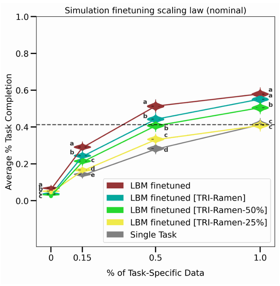
Original Figure 7 (PDF p. 10). Horizontal axis: fine-tuning data fraction. Vertical axis: mean TC across five unseen simulation tasks. Curves correspond to different pretraining mixtures.

At the same fine-tuning data fraction, more diverse pretraining data generally yield better performance, particularly when target-task data are scarce. The horizontal axis varies fine-tuning data. These limited subset experiments establish neither a universal scaling law nor benefits from increasing model parameter count.

Limitations

• Gains without fine-tuning are inconsistent. Pretrained LBMs do not consistently outperform single-task policies; the authors suggest this may partly reflect limitations in language guidance from the small language encoder.
• The experimental scope is limited. Results on a particular bimanual platform do not directly generalize to single-arm robots or arbitrary homes.
• Training randomness is not fully evaluated. Violin plots primarily capture evaluation uncertainty for fixed checkpoints, rather than variation across independent training runs.
• Pretraining contained a normalization bug. Some data used parameters from another source, and the main experiments were not all rerun. After correction, supplementary experiments improved performance under the tested simulation distribution shifts.
• Filtering stationary frames has mixed effects. Removing initial low-motion segments improved some single-task simulation policies but caused some pretrained models to select the wrong task more often. It was therefore not applied uniformly.

LeRobot Implementation and Application

The following comparison uses commit f5c9bc0. LeRobot MultiTask DiT follows the LBM conditional DiT approach, but its configuration, preprocessing, and training results should be interpreted separately.

Configuration Comparison

Component	TRI paper	Pinned LeRobot defaults
Objective	Diffusion noise prediction; DDIM sampling	diffusion; also supports flow_matching
Image and text backbones	CLIP; vision trainable, text frozen	Same approach; defaults to openai/clip-vit-base-patch16
DiT size	8 layers; hidden dimension 768	6 layers; hidden dimension 512; 8 attention heads
Observation history	2 frames	n_obs_steps=2
Action output	16 steps, each 20-dimensional	horizon=32; action dimension from the dataset
Execution segment	Execute 8 steps before replanning	n_action_steps=24; slice using the observation offset, then enqueue
Cameras	Standardized to 6 views; missing views zero-padded	Count inferred from input features; shared vision encoder by default
Normalization	Quantiles by source, relative timestep, and feature dimension	States and actions: MIN_MAX; images: MEAN_STD

By default, num_inference_steps=None falls back to num_train_timesteps=100, giving 100 denoising steps. Rotary position embeddings (RoPE) are enabled by default. Learnable absolute position embeddings are also supported; this version permits both simultaneously.

Parameter count depends on the camera count, layer count, and hidden dimension. The Boston Dynamics blog's 450M parameters, 48-step prediction horizon, and 24-step execution segment describe the Atlas configuration and do not apply to every LeRobot configuration.

Action Window and Execution Segment

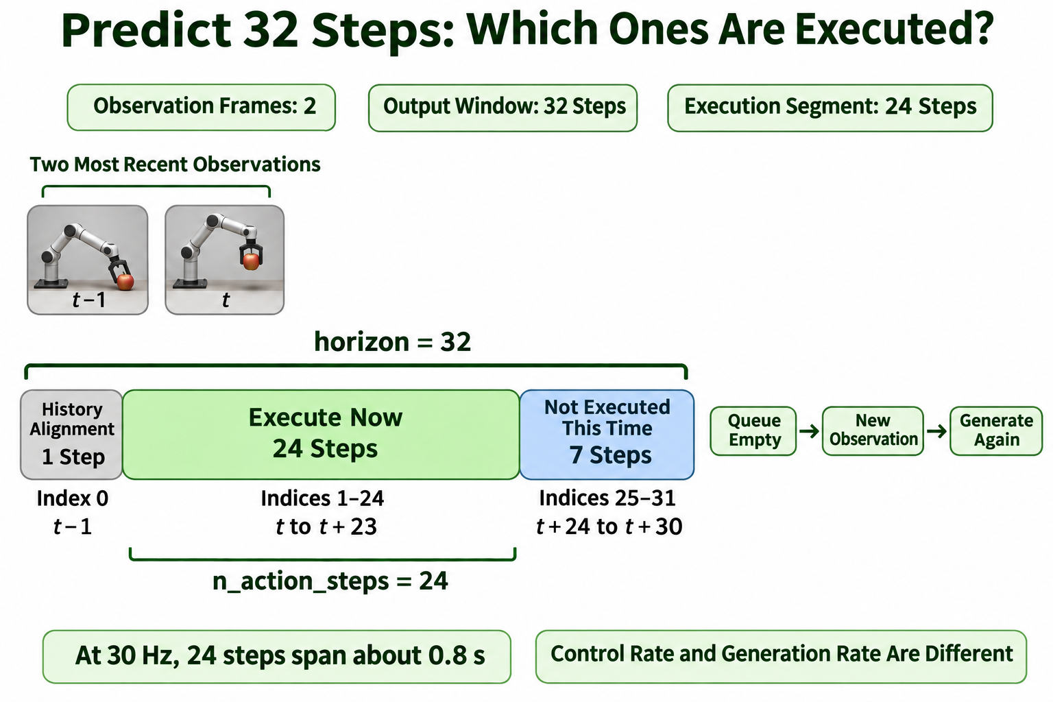
Teaching illustration based on action slicing in the pinned LeRobot implementation. The 32-step window and 24-step execution segment are this version's defaults.

With two observation frames, the action window starts at $t-1$. _generate_actions takes indices 1:25, placing 24 actions from $t$ through $t+23$ in the execution queue. Window length $H$, observation count $N_o$, and execution length $N_e$ must satisfy:

$$N_o-1+N_e\leq H,$$

For $N_o=2$, $N_e=24$, and $H=32$, this gives $2-1+24\leq32$.

When demonstration sampling and action execution both run at 30 Hz, 24 steps correspond to the illustrated 0.8 seconds; at 10 Hz, they span approximately 2.4 seconds. Shorter execution segments incorporate new observations sooner but require more frequent generation. Actual timing also depends on inference and communication latency; window parameters do not set the control frequency.

Training Initialization and the Paper's Conclusions

LeRobot can initialize its image and text encoders from pretrained CLIP weights and train an action policy on your own robot demonstrations. This does not provide TRI's robot multitask pretraining experience. Testing the paper's transfer benefits requires comparing single-task training with multitask pretraining followed by fine-tuning, while controlling target-task data, action interfaces, and test conditions.

For adaptation to reBot or SO-ARM101, first check dataset states, actions, cameras, timestamps, and task instructions, then validate the single-task control pipeline.

Interpreting the Conclusions

The paper uses a fixed policy architecture and controlled evaluation to test the benefits of multitask pretraining. On the evaluated tasks, pretraining followed by fine-tuning improves aggregate performance and reduces the target-task demonstrations needed for comparable performance. Some advantages become more pronounced when test conditions change.

The results support pretraining on diverse demonstrations within clear limits: gains depend on the task and fine-tuning conditions; better completion does not necessarily imply full success; and models without fine-tuning do not consistently outperform single-task policies. Understanding the contribution requires connecting action generation, experimental comparisons, and the scope of the evidence.