SEEED STUDIO · PAPER DEEP-DIVE

π₀-FAST — Efficient Action Tokenization

FAST: Efficient Action Tokenization for Vision-Language-Action Models

• Action tokenization
• DCT
• BPE compression
• Autoregressive policies

arXivRead the paper↗

Relationship to π0: The paper is titled FAST; π0-FAST is the policy trained using it. FAST is a tokenization method, FAST+ a pre-trained universal action tokenizer, and π0-FAST an autoregressive VLA using this representation. It shares the PaliGemma backbone approach with π0 but changes action generation; it is not merely a compression preprocessor added to π0's flow-matching expert.

Reading source: The original PDF, Sections I–VII and Appendices A–E, following the structure of the preceding π0 deep dive. Page numbers refer to physical pages of the 19-page PDF, from which the figures are extracted. Additional derivations and numerical examples are marked as explanations rather than attributed to the paper.

Prerequisites

VLAs and Action Tokenization

Explanation: A VLA converts a visible scene and a language task into robot controls. For T-shirt folding, images locate the shirt and grippers, language defines the objective, state describes the arms, and the model predicts future arm and gripper actions.

This paper uses action chunking: predict $H$ future steps rather than only one. Define:

$A_t=[a_t,a_{t+1},\ldots,a_{t+H-1}]\in\mathbb R^{H\times D},\qquad o_t=(I_t^1,\ldots,I_t^m,\ell_t,q_t)$

Here $t$ is robot control time, $a_t$ a $D$-dimensional action, and $H$ the horizon. $I_t^i$ is image view $i$, $m$ the camera count, $\ell_t$ the instruction, and $q_t$ proprioception. The policy learns $\pi_\theta(A_t\mid o_t)$, where $\theta$ denotes network parameters.

Paper: Chunks are primarily one second long. Thus $H$ depends on control rate: 15 at 15 Hz, 20 at 20 Hz, and 50 at 50 Hz. Do not assume π0's $H=50$ for every dataset here.

Action tokenization maps a continuous chunk to discrete symbols:

$\mathcal T(A_t)=[z_1,z_2,\ldots,z_n],\qquad z_k\in\{0,\ldots,V-1\}$

$\mathcal T$ is the tokenizer, $z_k$ an action-token ID, $V$ vocabulary size, and $n$ compressed sequence length. Equally shaped chunks can produce different $n$, just as equally long sentences can have different subword counts.

Caution: A token ID is not a joint angle. A FAST token need not correspond to one timestep, joint, or complete action. Generate the sequence first, then decode it to a continuous chunk.

Pointwise Binning, π0 Flow Matching, and FAST

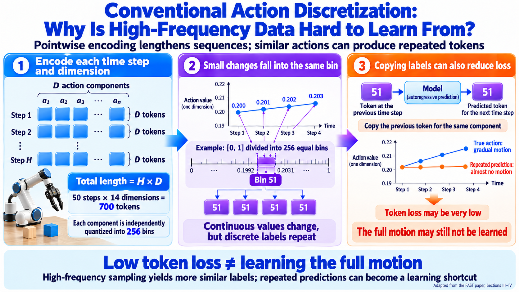
Conventional binning independently quantizes each timestep and action dimension. A common configuration discussed in the paper uses 256 uniform bins:

D action components at step 1 → D tokens
D action components at step 2 → D tokens
……
D action components at step H → D tokens
Total: H × D tokens

High-rate data then produces long sequences with highly similar neighboring values. Copying repeated tokens can reduce loss without learning the overall motion.

Minimal example: Values $[0.200,0.201,0.202,0.203]$ may all fall into one coarse bin. Repeating the previous token predicts many labels correctly but fails to express the steadily changing trajectory.

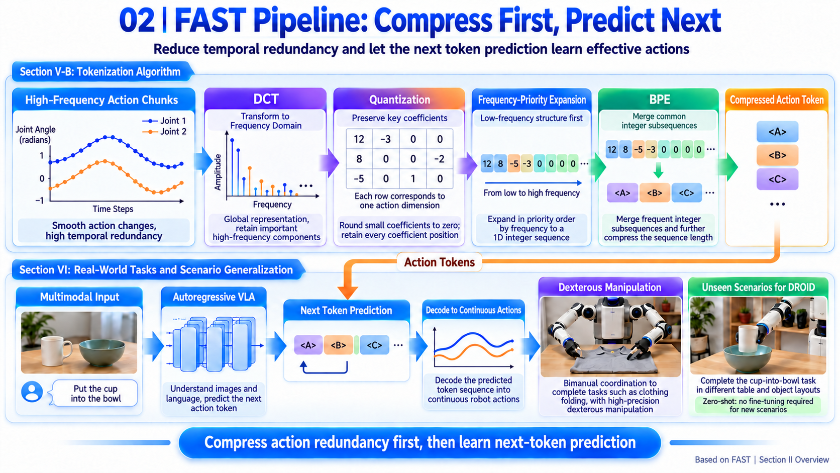
FAST uses:

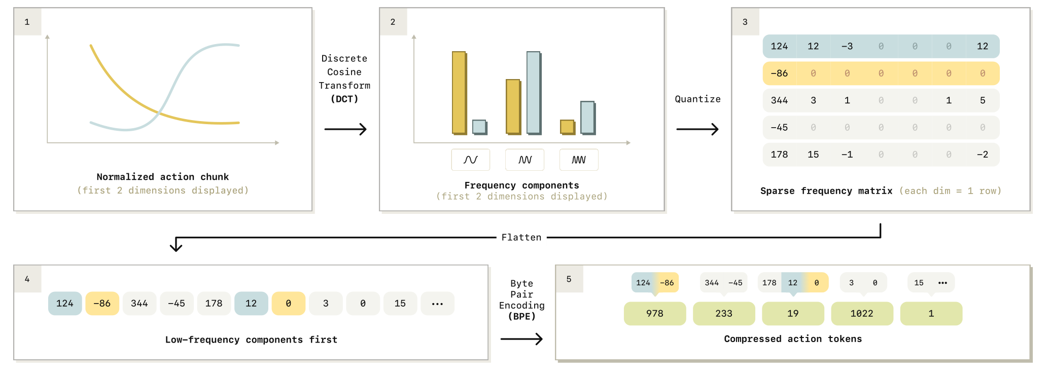
Continuous chunk → frequency coefficients → quantization → frequency-first flattening → BPE
          → fewer action tokens → autoregressive VLA prediction → continuous-chunk decoding

The discrete cosine transform (DCT) expresses a trajectory as cosine components at different frequencies; byte-pair encoding (BPE) merges common integer subsequences. Predicting this compressed trajectory representation removes redundant supervision.

Aspect	Pointwise autoregressive VLA	Original π0	π0-FAST
Representation	Discrete value per timestep and dimension	Continuous chunk	Compressed discrete tokens for a chunk
Objective	Next-token prediction	Conditional flow matching	Next-token prediction
Generation	Sequentially generate $HD$ tokens	Iteratively update the complete chunk with an expert	Generate $n$ compressed tokens, then decode
High-rate data	More tokens and repetition	Continuous generation avoids dimension-by-dimension decoding	Compress temporal redundancy and shorten the output
Main limitation	High-rate dexterity can be difficult to learn	Requires a dedicated continuous expert	Lossy quantization; autoregressive inference can still be slow

Paper: Table I reduces a one-second, 50 Hz, 14D T-shirt chunk from 700 pointwise tokens to an average of 53 FAST tokens. Decoding still yields 50 × 14 actions; robot control does not become “53 tokens per second.”

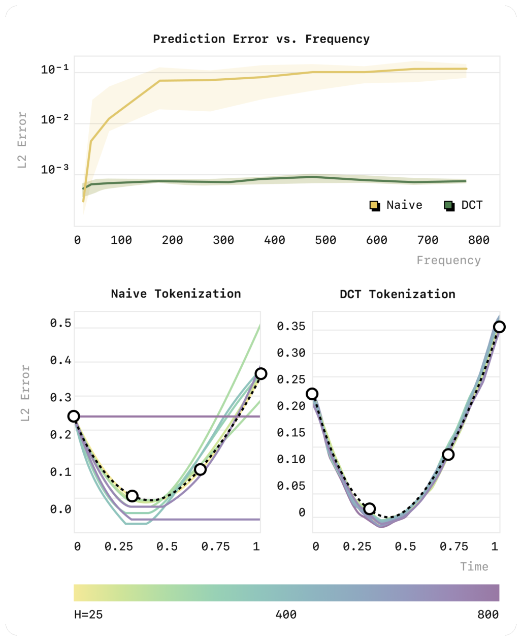
Figure 2: predictions of the same cubic spline at different sampling densities. Yellow is pointwise binning; green is DCT. The lower color scale goes from light yellow to purple as sample count $H$ increases from 25 to 800. From original Figure 3, PDF page 3.

Reading the figure: Four input points define the same kind of interpolation target while density increases. Pointwise-tokenization error grows, eventually approaching a constant prediction; DCT error remains low. Learning can fail because of representation rather than a harder task. The 25–800 values are synthetic samples per sequence, not real robot control frequencies.

Training, Inference, and Evaluation

Stage	Inputs and operations	Output and criterion
Tokenizer training	Normalize actions, apply DCT and quantization, and learn BPE from integer sequences.	Encoding/decoding rules; compression and reconstruction error.
Policy training	Condition on images, language, and state; encode future demonstrated actions as FAST labels.	Cross-entropy optimization and VLA weights.
Policy inference	Generate tokens, reverse BPE, dequantize, and apply inverse DCT.	Continuous chunks for the controller.
Robot evaluation	Execute specified tasks and starting conditions.	Task success or normalized progress.

Paper: Evaluation includes six real-robot tasks/settings and one simulation benchmark, plus separate offline FAST+ compression tests across embodiments. Compressing humanoid data is not the same as training and physically validating a humanoid policy.

Caution: Token loss, reconstruction error, and task score are distinct. A key finding is that repetitive labels can produce low training loss while trajectories and robot behavior remain poor.

---

Abstract

Translation

Autoregressive sequence models, including Transformer VLAs, can represent complex generalizable robot behavior, but require a tokenizer to map discrete predictions to continuous actions. The authors find that simple per-dimension, per-timestep binning performs poorly on high-frequency dexterous data.

They propose Frequency-space Action Sequence Tokenization (FAST), using DCT-based compression to let autoregressive VLAs learn high-frequency dexterous tasks where standard discretization fails.

FAST+ is a universal tokenizer trained on one million real-robot action sequences, usable as a black-box tokenizer across different action spaces and control frequencies.

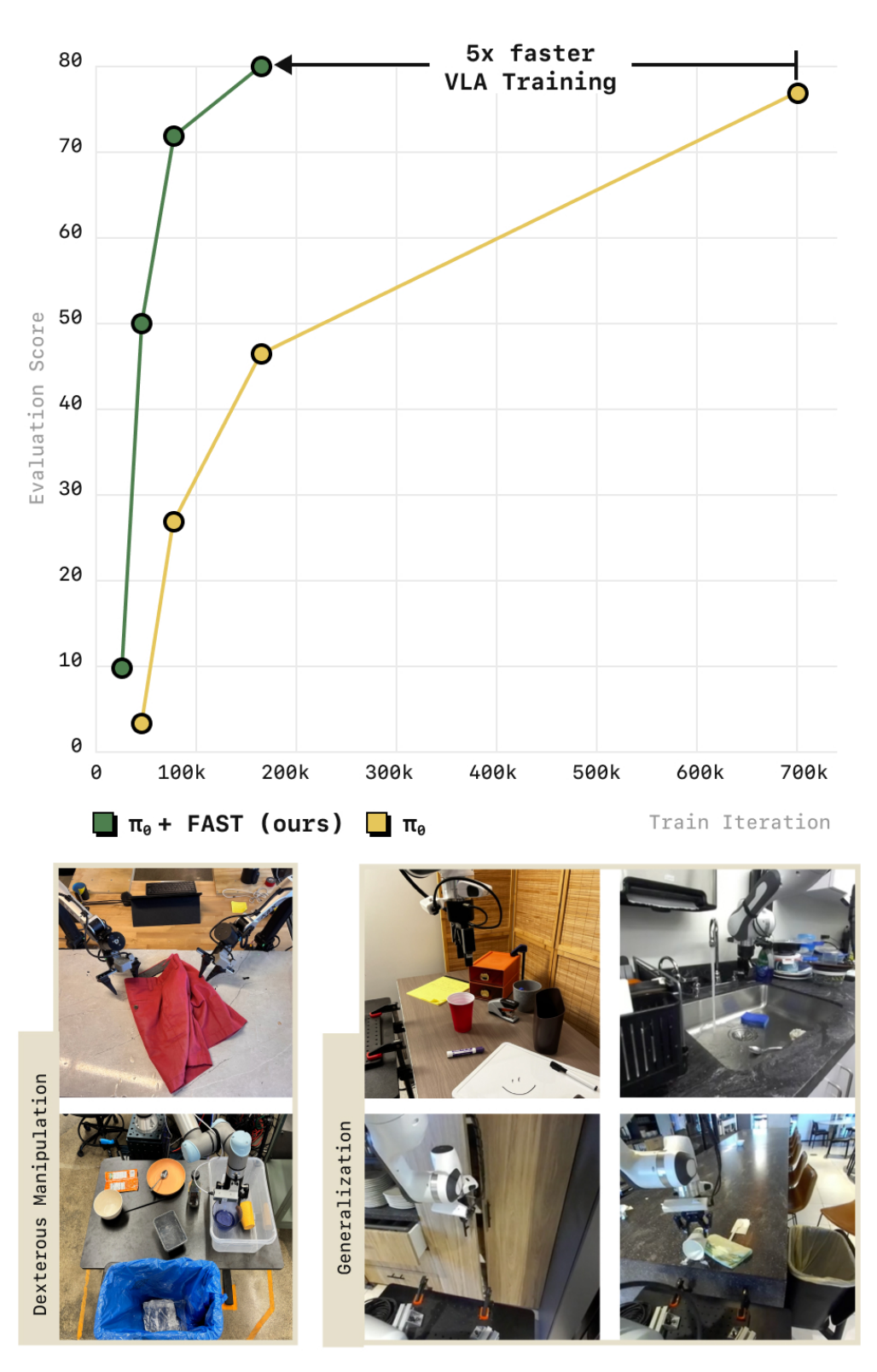
Combined with the π0 VLA approach, FAST scales to 10,000 hours of robot data, matches diffusion-style VLA performance, and reduces training time by up to five times.

Commentary

• Motivation: High-rate actions contain repeated information. Pointwise tokens spend prediction effort on labels with little new motion supervision.

• Core change: Change the learning-target representation before training the policy. FAST compresses trajectory information without lowering execution frequency or discarding control points.

• Why it can work: DCT concentrates trajectory shape, quantization creates compressible coefficients, and BPE shortens common combinations. All three contribute to the final tokens.

• Meaning of “universal”: FAST+ avoids retraining a dataset-specific BPE vocabulary, but still requires compatible normalization, dimensions, and horizons. Its million training samples are mainly one-second chunks, not a million complete task episodes.

• Scope of “five times”: Large-scale policy experiments reduce required GPU hours by up to about five times. This is not faster inference: v1 reports around 750 ms per π0-FAST chunk versus usually under 100 ms for π0.

---

Introduction

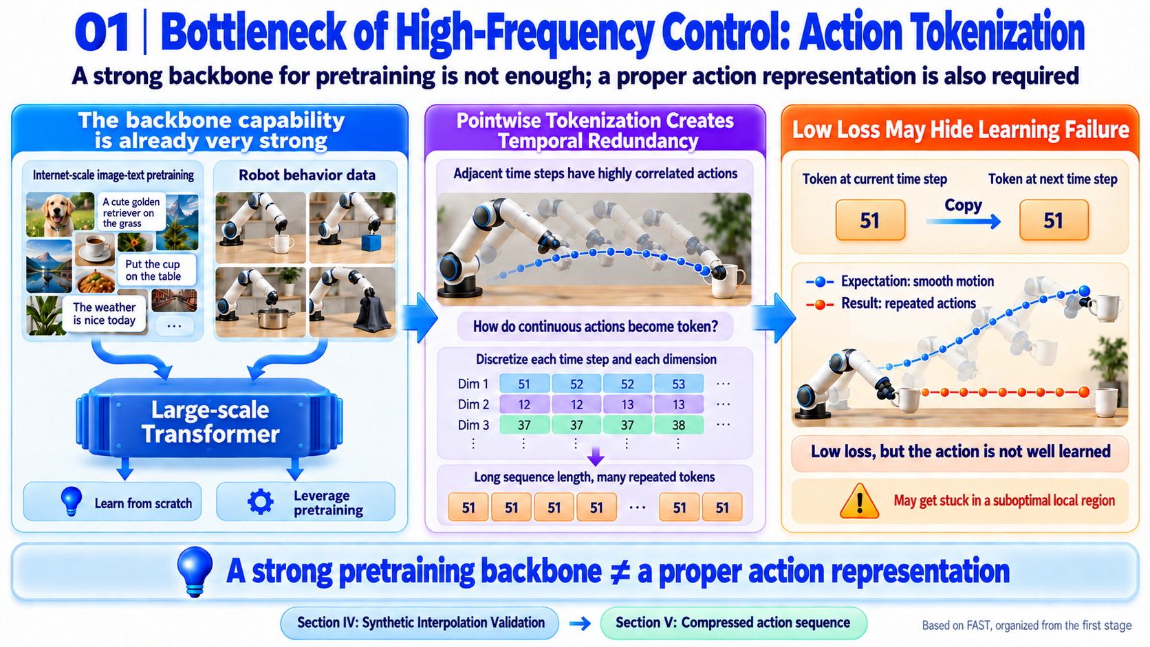
Paragraph 1: Locate the Bottleneck in Tokenization

• Main point: Large Transformers can learn robot behavior from scratch or use image-text pre-training, but actions must be tokenized. Pointwise binning struggles on dexterous high-rate tasks because copying correlated recent values achieves low loss and can trap learning in a poor local optimum.

• Problem: A powerful backbone does not guarantee useful action learning; target representation can limit the supervision.

• Setup: Section IV studies sampling density with synthetic interpolation; Section V proposes compression.

Paragraph 2: Compress First, Predict Second

• Main point: Inspired by language tokenization, FAST uses DCT for continuous robot signals. Standard next-token prediction then learns previously failing tasks and supports a DROID policy used through language in unseen settings.

• Problem: If temporal redundancy is the obstacle, reduce label redundancy rather than only increasing network capacity.

• Setup: Section V-B gives the algorithm, and Section VI evaluates real tasks and DROID generalization.

Paragraph 3: Universal Tokenization and Large-Scale Policies

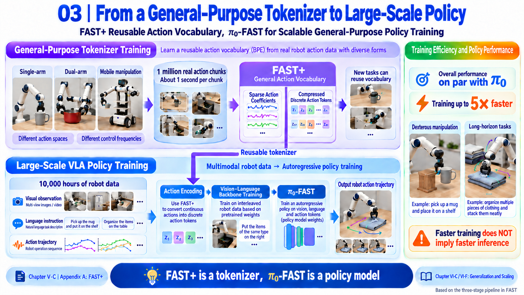
• Main point: FAST+ learns a vocabulary from one million sequences covering single-arm, bimanual, mobile, and varied control interfaces and frequencies. π0-FAST scales autoregression to 10,000 hours with less training time than the diffusion-style comparison.

• Problem: Retraining a tokenizer for every robot adds overhead, and the method must scale beyond individual datasets.

• Setup: Section V-C and Appendix A describe FAST+; VI-C tests universality and VI-F large-scale policies.

Caution: The introduction contains three main paragraphs, with the first spanning pages 1–2. Page breaks and figure captions are not extra paragraphs. Claims about the “first” DROID result reflect the authors' assessment at publication, not a survey of later work.

---

Related Work

• Text, image, and audio tokenization: Text BPE merges frequent subsequences; other modalities use learned quantization or frequency representations. FAST applies the representation-and-compression principle to continuous action chunks. DCT is analytic; only the BPE vocabulary is learned.

• VLAs: RT-2 and OpenVLA transfer image-text knowledge to control but commonly use pointwise action bins. FAST changes outputs so an autoregressive backbone can learn high-rate dexterity; continuous-flow π0 is a key comparison.

• Action representations: Semantic subtasks and keypoints may depend on hand-designed controllers; binning directly represents controls but has temporal redundancy; regression and diffusion heads change output mechanisms. FAST retains discrete sequence prediction. The learned compression comparison uses finite scalar quantization (FSQ). FAST needs no neural encoder and performs better on the tested high-fidelity reconstructions and dexterous tasks, not necessarily every learned tokenizer.

---

π0-FAST Policy System and Experimental Platforms

Goals and Components

FAST is an action-processing method, not new teleoperation hardware. This system section explains how tokenization, the VLA, control, and evaluation fit together.

Goals are to compress high-rate actions while retaining fine trajectories, reuse autoregressive VLM training, support varied action spaces, enable easy tokenizer training/reuse, and scale across embodiments.

Component	Paper configuration	Role
FAST / FAST+	DCT, quantization, frequency-first flattening, BPE	Encode chunks as predictable symbols and decode them.
π0-FAST backbone	PaliGemma-3B	Encode images/language and autoregressively generate action tokens.
Backbone-transfer comparison	OpenVLA based on Prismatic 7B	Test whether benefits extend beyond PaliGemma.
Images	Two or three $224\times224$ views	One external view plus one wrist view per arm.
Proprioception	256-bin discretization, then integer-text tokenization	Supply the current robot state.
Execution	Platform-specific low-level controllers	Send decoded continuous values to joints, grippers, and other controls.

Paper: All policy weights are fine-tuned. Each image is encoded separately, then visual tokens are concatenated. Image size and textual state encoding are specified in Appendix C rather than inferred from π0.

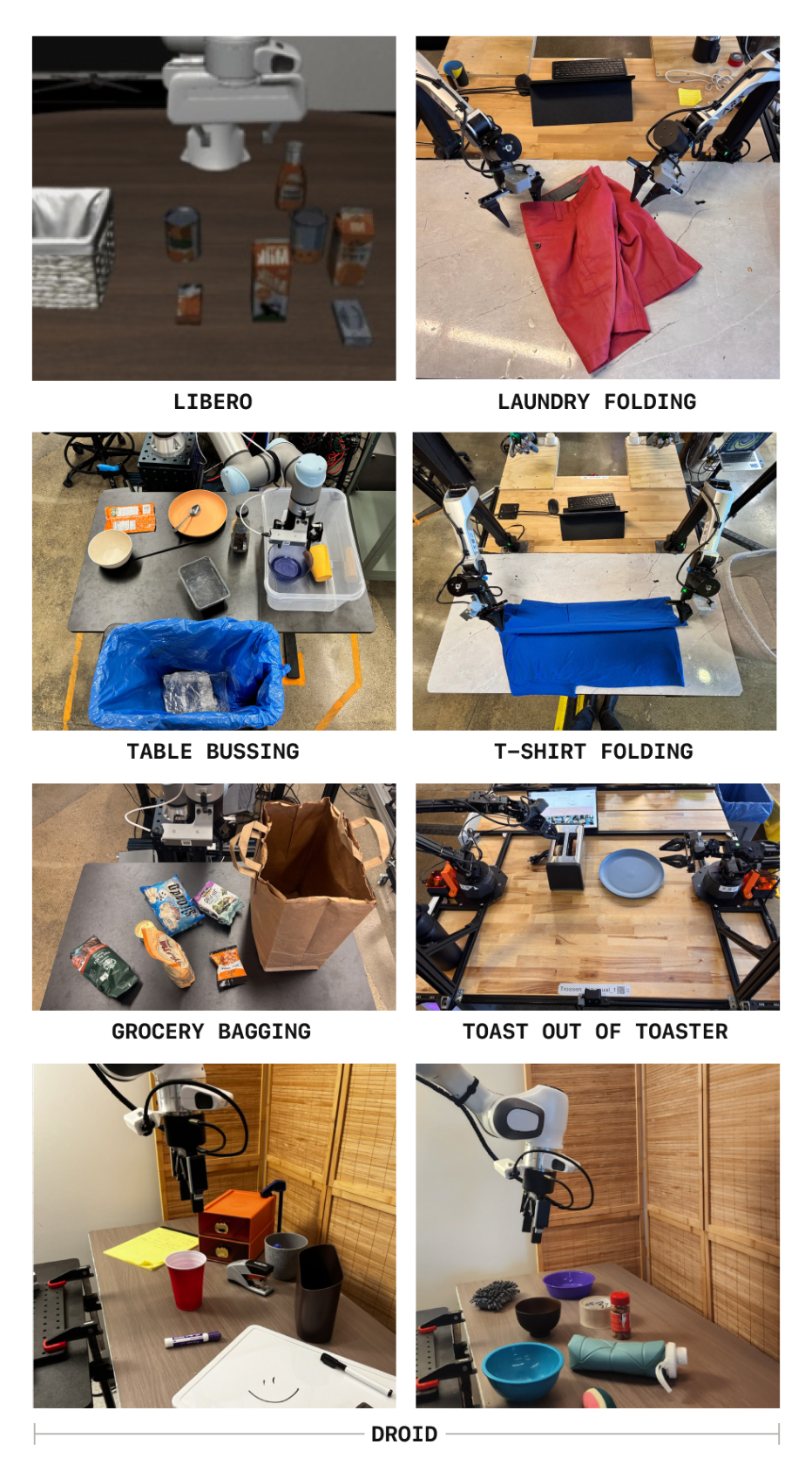
Task / setting	Platform and control rate	Capability tested
LIBERO	Simulation	Spatial, object, goal, and long-horizon generalization.
Table bussing	Single UR5/UR5e, 20 Hz	Grasp, sort, and store 12 objects.
T-shirt folding	Bimanual ARX, 50 Hz	Precisely grasp and fold a flat shirt.
Grocery bagging	Single UR5/UR5e, 20 Hz	Bag seven objects without collapsing or tearing the bag.
Toast out of toaster	Bimanual Trossen Viper-X, 50 Hz	Remove two toast slices and place them on a plate.
Laundry folding	Bimanual ARX, 50 Hz	Retrieve, spread, fold, and stack garments from a basket.
DROID zero-shot tabletop tasks	Franka data and deployment, 15 Hz	Follow language for placement, wiping, drawer operations, and related tasks in new scenes.

Caution: High control frequency means many control points per second; high frequency in DCT means rapid variation along a trajectory. Smooth 50 Hz motion can still be dominated by low-frequency coefficients. Neither is the full model's inference rate.

Connecting Encoding, Prediction, and Execution

The complete workflow is:

Demonstrations → one-second future chunks → normalization and FAST → action-token labels
Current images + language + state → VLM prefix → learn action-token prediction
                                      ↓ after training
New observations → autoregressive tokens → FAST decoding → continuous chunk → execute
                                                                  ↓
                                                          observe and predict again

FAST encodes only action targets; it does not interpret images or apply DCT to current proprioception. During training, the model sees ground-truth previous action tokens; at inference, it sees its own generated tokens.

Paper: Action symbols replace rarely used slots in the VLM vocabulary, reusing discrete outputs without a π0-style flow expert. OpenVLA experiments still modify multi-image inputs and chunk outputs. Compatibility with autoregressive backbones does not mean every existing robot codebase needs no adaptation.

Execution timing: DROID predicts 15 steps and executes eight or 15 open-loop before updating observations. At 15 Hz, these cover about 0.53 or one second of control points, not total wall-clock cycles including inference and communication. v1 does not specify one execution length for every platform.

Rationale: Chunks retain trajectory coherence; compression makes high-rate labels learnable; autoregressive outputs let pre-trained image-text weights participate directly. Controllers receive continuous values, not BPE IDs.

Data, Capabilities, and Results

Dataset Scale and Configuration

Use	Scope	Distinction
FAST+ tokenizer training	About one million one-second real-action chunks	Learns BPE, not VLA visual understanding.
FAST+ coverage	Single-arm, bimanual, mobile; joint, world-frame end-effector, and camera-frame end-effector controls; varied frequencies	One robot can contribute multiple action parameterizations.
Large-scale policy	π0 mixture: 903M internal timesteps, with open data receiving 9.1% mixture sampling weight	Open sources include Bridge v2, DROID, and OXE; 9.1% is not a raw-data-volume fraction.
DROID-specific policy	75k successful episodes, about 21M samples	Light filtering and removal of all-zero idle actions; policy training is still required.
DROID training	Batch 256, 240k iterations, about three epochs	Appendix D reports about four days on eight H100s for this configuration.

Paper: FAST+ training pads actions to 32 dimensions. This aligns tokenizer data, not every policy's output size, and differs from π0's 18D interface. New platforms still need their effective action dimensions defined.

DROID uses one external and one wrist image. Training randomly chooses between two available external cameras and three language annotations per episode, without camera calibration information. Controls are joint velocities and absolute gripper position. New-view deployment does not eliminate the need to configure coordinates and control interfaces.

Compression: Fewer Tokens, the Same Action Horizon

These one-second results reproduce Table I. Compression is pointwise token count divided by average FAST count at similar reconstruction error.

Dataset / task	Dimension $D$	Rate and horizon $H$	Pointwise tokens	Average FAST tokens	Compression
BridgeV2	7	5 Hz, 5 steps	35	20	1.75
DROID	7	15 Hz, 15 steps	105	29	3.6
Table bussing	7	20 Hz, 20 steps	140	28	5.0
T-shirt folding	14	50 Hz, 50 steps	700	53	13.2

Interpretation: Increasing control points does not necessarily add proportionally new motion information. About 30 tokens per arm per second is an empirical observation here, not a fixed length.

Version check: Appendix Table III uses some different-dimensional offline datasets, including 8D DROID Joint and table bussing, while Table I lists 7D. The Table I convention is retained rather than merging different parameterizations into one specification.

Evaluation: Success and Progress Are Different

Task	Evaluation
LIBERO	Binary episode success; four suites jointly trained on about 270k samples for 40k iterations.
Table bussing	Fraction of 12 objects correctly placed in the trash or storage container.
T-shirt folding	Human-judged folding success across five seen shirts.
Grocery bagging	Fraction of seven objects placed in the bag.
Toast removal	One point per slice removed and one per slice plated; four points total, then normalized.
Laundry folding	Human-judged garment folding and stacking, with five random garments in the basket.
DROID quantitative tests	44 trials per policy, with task-specific progress points such as correct grasp and destination.

Version check: The main text calls LIBERO's fourth suite Libero-10; the appendix calls it Libero-Long. It is described as the long-horizon suite here. Appendix E says 16 DROID tasks, while Table II lists 17 names; trial counts still sum to 44. The discrepancy is preserved rather than silently resolved.

Evidence boundary: Deployments across Berkeley, Stanford, and the University of Washington are additional qualitative demonstrations without reported success rates. Zero-shot means no further training for the new deployment scene, not no DROID training. FAST+ vocabulary training also includes data from real evaluation tasks, so Figure 6 does not show both tokenizer and policy completely unfamiliar with every task.

Comparing Tokenizers

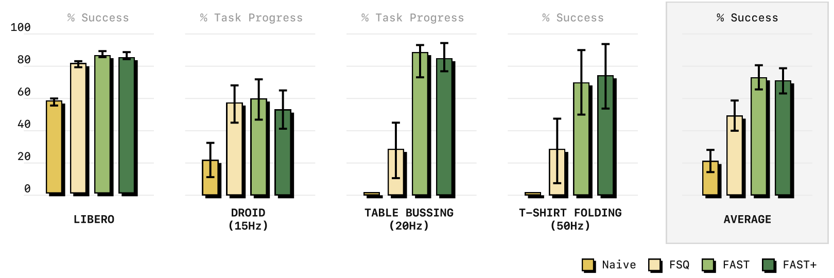
On 20 Hz table bussing and 50 Hz T-shirt folding, pointwise binning makes little progress, while FAST and FAST+ learn useful policies. FSQ supports the value of compression but generally trails FAST on these dexterous tasks. Universal FAST+ is close to dataset-specific FAST, supporting its use as a default.

Caution: The figure averages different task scores, so it is not a uniform average success rate. Error bars also limit conclusions about small differences between similar bars.

Single-Dataset Comparison with π0

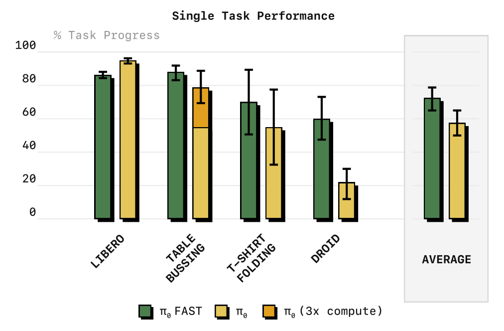
• On smaller datasets such as LIBERO and T-shirt folding, the authors judge performance comparable.

• On large table-bussing data, FAST reaches strong performance sooner; π0 takes about three times as many steps to approach it.

• On DROID, π0-FAST follows language more reliably while flow-matching π0 often ignores it; the paper does not establish the underlying cause.

Explanation: Teacher forcing computes losses for output positions in parallel during training; autoregressive inference remains sequential. Faster training and slower inference can coexist. These results do not establish universal autoregressive superiority.

Large-Scale Generalists and Compute-Matched Comparison

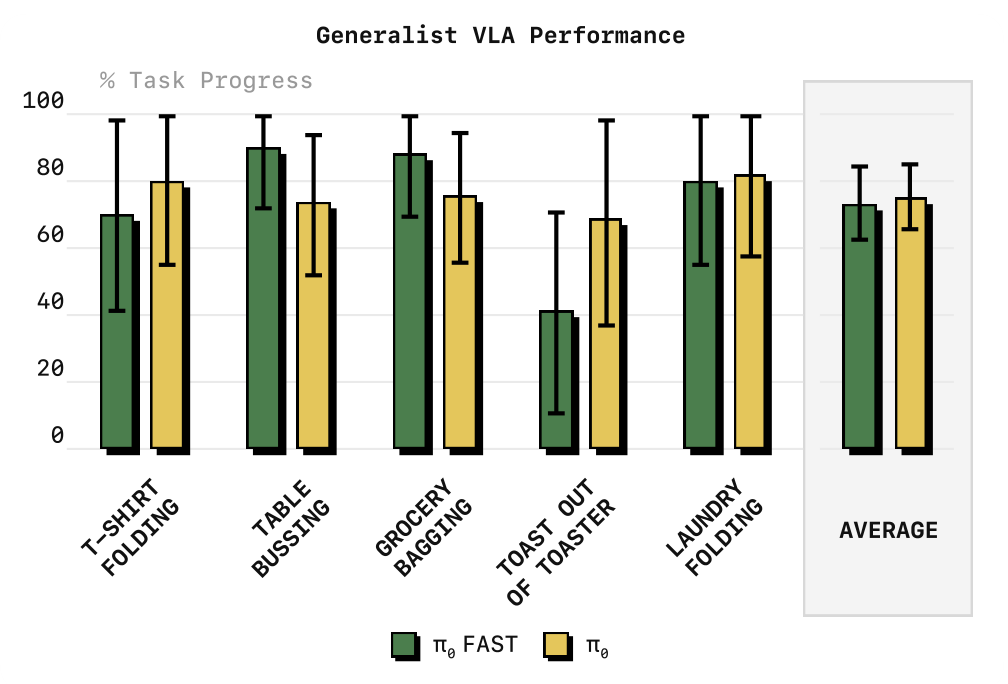
π0-FAST has similar overall performance to π0 across folding, bussing, bagging, toast, and laundry. Individual tasks vary; toast does not support a claim of universal FAST superiority. The evaluated π0-FAST uses about one-fifth as many GPU hours.

Caution: VI-F broadly describes zero-shot comparison, but Appendix E specifies high-quality task fine-tuning for laundry after large-scale pre-training. Bagging and toast use pre-trained models directly. Not every Figure 6 task is free of task-specific fine-tuning.

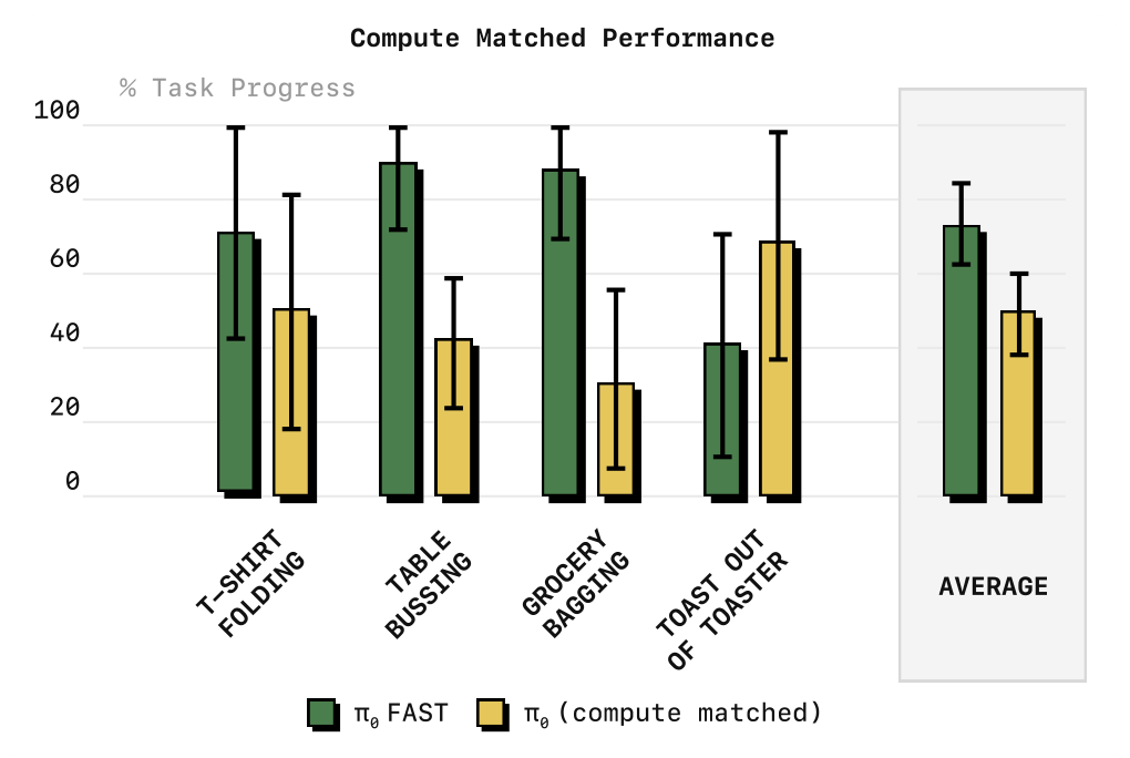
Compute matching more directly supports faster convergence: FAST has a higher overall mean and clear bussing/bagging gains, while still trailing on toast. This is evidence of training efficiency, not stronger final capability on every task.

Deployment boundary: On RTX 4090, VI-E reports usually under 100 ms for π0 and about 750 ms for π0-FAST per one-second chunk. FAST decodes roughly 30–60 tokens through the full language backbone; π0 repeats mainly its smaller 300M expert for ten flow updates. Static tasks tolerate this latency, but dynamic tasks and inference optimization remain future work.

---

Frequency-Space Tokenization and Autoregressive Policy Modeling

Mechanism 1: Express a Trajectory with DCT

Problem and Intuition

Neighboring control points on smooth trajectories are similar. Independent targets grow with sampling rate without adding much information. DCT instead describes which cosine shapes combine, and with what amplitudes, to form the trajectory.

A few low-frequency coefficients often describe smooth global shape; higher frequencies represent rapid changes and detail. DCT itself neither discards high frequencies nor imposes a fixed low-pass filter. Full DCT and inverse DCT are reversible; quantization introduces the loss.

Formal Expression

Explanation: The paper applies DCT independently along each action dimension. An orthonormal DCT-II convention is used below for clarity, without claiming the pseudocode specifies that normalization.

For normalized chunk $X\in\mathbb R^{H\times D}$:

$C_{k,d}=\alpha_k\sum_{j=0}^{H-1}X_{j,d} \cos\left[\frac{\pi}{H}\left(j+\frac12\right)k\right]$

$\alpha_0=\sqrt{\frac1H},\qquad \alpha_k=\sqrt{\frac2H}\quad(k>0)$

$j$ indexes time within the chunk, $d=1,\ldots,D$ action dimensions, and $k=0,\ldots,H-1$ frequency. $C\in\mathbb R^{H\times D}$ is the coefficient matrix. $k=0$ is constant; higher $k$ varies faster. DCT acts along time, not across joints.

The corresponding inverse is:

$X_{j,d}=\sum_{k=0}^{H-1}\alpha_k C_{k,d} \cos\left[\frac{\pi}{H}\left(j+\frac12\right)k\right]$

Every timepoint depends on multiple frequencies; one frequency coefficient usually affects the whole chunk.

Minimal Numerical Example

Explanation: Let $H=4,D=2$, with illustrative normalized actions:

$X=\begin{bmatrix} 0.2&0.0\\ 0.2&0.1\\ 0.2&0.2\\ 0.2&0.3 \end{bmatrix} \quad\Longrightarrow\quad C\approx\begin{bmatrix} 0.4&0.3\\ 0&-0.2230\\ 0&0\\ 0&-0.0159 \end{bmatrix}$

The constant first dimension needs only one nonzero constant coefficient. The increasing second dimension is mostly represented by the constant and first varying component, with a small highest-frequency coefficient. There are still four timesteps and two dimensions; only the coordinate representation changes.

Why it helps: Dense samples of smooth motion add similar points without necessarily adding important frequencies. Concentrating shared information makes compression into fewer informative tokens possible.

Scale and limits: Chunks are usually about one second. $H=1$ offers no temporal redundancy; short chunks limit compression, while long chunks increase the horizon and, if executed open-loop, delay feedback. Abrupt contact or gripper transitions may require higher frequencies; a few low frequencies cannot represent every action accurately.

Mechanism 2: Quantization, Frequency-First Ordering, and BPE

Why DCT Alone Is Insufficient

DCT still produces $HD$ real coefficients. Tokenizing each separately does not shorten the sequence, and near-zero coefficients create repeated labels. FAST therefore adds quantization and BPE.

Per-Dimension Percentile Normalization

Paper: Map each training-data dimension's 1st and 99th percentiles to $-1$ and $1$, reducing scale differences and outlier influence.

Explanation: For a nondegenerate dimension:

$X_{j,d}=2\frac{A_{t}[j,d]-L_d}{U_d-L_d}-1$

$L_d$ and $U_d$ are the 1st and 99th percentiles, respectively; $A_t[j,d]$ is the physical action component, and $X_{j,d}$ its unitless normalized value. If $L_d=0,U_d=2$ for a joint, physical actions $0,1,2$ map to $-1,0,1$.

Caution: Mapping percentiles does not force every value into $[-1,1]$. Follow the implementation for clipping and degenerate $L_d=U_d$; v1 does not detail them. Save training statistics for deployment rather than recomputing percentiles on each predicted chunk.

Scale and Round to Create Compressible Integers

$Q_{k,d}=\operatorname{round}(\gamma C_{k,d}),\qquad \widehat C_{k,d}=\frac{Q_{k,d}}{\gamma}$

$Q$ is the integer matrix, $\gamma>0$ the scale, and $\widehat C$ reconstructed coefficients. Larger $\gamma$ makes the grid finer, usually improving reconstruction but potentially increasing tokens; smaller values zero more small coefficients and compress more at greater error.

Paper: Dataset-specific experiments use $\gamma=10$ and vocabulary $V=1024$, with limited sensitivity in the tested range. These are not universal settings for arbitrary action spaces.

Continuing the example with $\gamma=10$:

$Q=\begin{bmatrix} 4&3\\ 0&-2\\ 0&0\\ 0&0 \end{bmatrix}$

The highest-frequency $-0.0159$ becomes zero, while $-0.2230$ becomes $-2$. No rule keeps only the first two frequencies; any sufficiently large coefficient can remain nonzero.

Explanation: Ordinary rounding gives $\|\widehat C_{k,d}-C_{k,d}\|\leq 1/(2\gamma)$. This bounds one coefficient's error, not physical joint error directly, which also depends on inverse transformation, action scale, and clipping.

Frequency-First Ordering Prioritizes Global Shape

Before BPE, FAST orders coefficients by increasing frequency, then by action dimension within each frequency:

$u=[Q_{0,1},\ldots,Q_{0,D},Q_{1,1},\ldots,Q_{1,D},\ldots,Q_{H-1,D}]$

$u$ contains $HD$ integers. In the example:

Frequency 0, two dimensions: 4, 3
Frequency 1, two dimensions: 0, -2
Frequency 2, two dimensions: 0, 0
Frequency 3, two dimensions: 0, 0
Flattened: 4, 3, 0, -2, 0, 0, 0, 0

Paper: Frequency-first ordering gives more stable rollouts than dimension-first ordering by predicting global low-frequency shape first. The original $D\times H$ matrix calls this column-major; this guide's $H\times D$ convention makes it row-major. The semantic ordering matters, not the row/column label.

BPE Merges Common Integer Subsequences

BPE learns frequent adjacent symbol combinations and adds them to a finite vocabulary. An illustrative vocabulary might merge $[0,0,0,0]$ or $[4,3]$ into individual tokens, shortening the eight-integer example.

Explanation: Actual merge rules and IDs depend on training data; these are not the paper's literal vocabulary. A token can span dimensions or neighboring frequencies, and decoding expands it back into integers.

Key distinction: Rounding coefficients is lossy; BPE is lossless on the quantized integer sequence. Zero positions are preserved and compressed, not removed. Otherwise inverse transformation would lose their frequency and dimension locations.

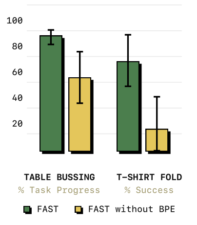
Reading the ablation: Without BPE, DCT still concentrates information and beats pointwise binning, but repeated zero tokens dilute supervision and add decoding steps. Performance drops on both real tasks, supporting separate contributions from DCT and BPE.

Modeling Demonstrations and Reusing FAST+ across Embodiments

One Observation Can Have Several Valid Actions

A person may grasp either shirt corner or unfold it differently. Direct mean-squared regression can average valid alternatives into an invalid middle path. π0 models a continuous distribution; π0-FAST models probabilities over compressed tokens.

Autoregressive factorization:

$p_\theta(z_{1:n}\mid o_t) =\prod_{k=1}^{n}p_\theta(z_k\mid o_t,z_{<k})$

$z_{1:n}$ is the FAST sequence and $z_{<k}$ its prefix before token $k$. Each step predicts vocabulary probabilities rather than averaging physical action values; the complete sequence decodes to a trajectory.

Caution: FAST has no CVAE encoder, noisy Gaussian action chunk, or flow-time input like π0. This section explains demonstration modeling without importing ACT or π0 modules. Coverage still depends on data, quantization fidelity, and learning.

Why Repeated High-Rate Labels Weaken Learning

Explanation: When adjacent values barely change, the next token's conditional entropy can be low:

$\mathrm H(Z_k\mid Z_{<k},o_t)$

$Z_k$ is a random action token and $\mathrm H$ conditional entropy, distinct from horizon $H$. A predictable prefix explains much of the next label, so repetition can score well without sufficient image or task dependence.

This information perspective explains the synthetic and high-rate results; it is not proof that every binned policy fails or fewer tokens always help. Severe compression loss can still produce incorrect behavior.

A Universal Vocabulary with FAST+

FAST's analytic steps transfer across datasets, but a dataset-specific BPE vocabulary does not necessarily do so. FAST+ learns broader coverage from about one million cross-embodiment chunks:

Multiple robots, action spaces, and control rates
→ Normalize for each data configuration
→ Pad training actions to 32 dimensions
→ DCT, quantization, frequency-first flattening
→ Train BPE on the pooled integer sequences
→ Reusable FAST+ tokenizer

The vocabulary learns common coefficient patterns and zeros, not camera semantics or a robot's complete kinematic controller. A new policy still needs image, language, state, and action data to learn what to do. Universal tokenization and generalist control are different levels.

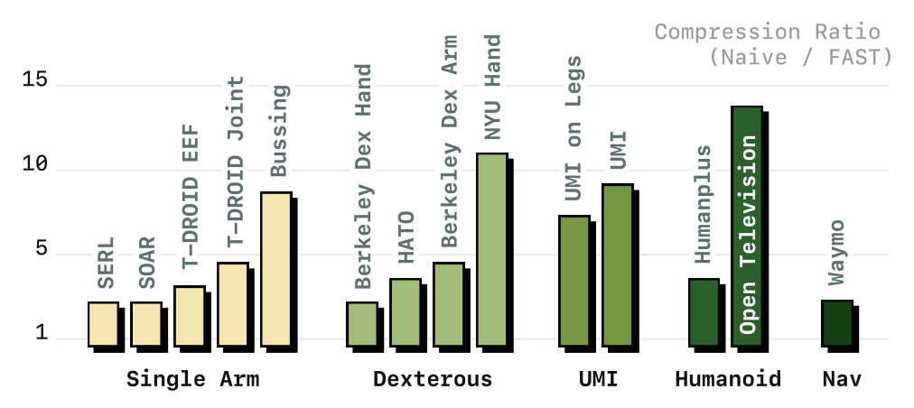
Reading the figure: FAST+ compresses varied shapes, dimensions, and frequencies. VI-C calls the tests unseen data, while Table III includes versions of platforms/tasks also named in training. “Unseen” is therefore retained at the paper's data-split level, not extended to every robot category.

Boundary: Figure 10 is offline compression, not humanoid locomotion, dexterous-hand, or driving-policy success. Section VII notes that physical policies are mainly validated on stationary manipulators. Table III includes 40D humanoid data, so 32D training padding is not a mathematical maximum for the method.

Training, Encoding, and Decoding the Tokenizer

Tokenizer Training

For demonstration chunks $\{A^{(s)}\}$, with sample index $s$:

1. Compute and save per-dimension percentile statistics for each data configuration.

2. Normalize to $X^{(s)}$ and apply DCT along time independently per dimension.

3. Quantize to integer $Q^{(s)}$ using fixed $\gamma$.

4. Flatten in frequency-first order to $u^{(s)}$.

5. Train fixed-size BPE on all integer sequences to obtain vocabulary and merge rules $\Phi$.

Paper: BPE is the only learned tokenizer component. A specific vocabulary usually trains in minutes, not the days or longer needed for a VLA. DCT and quantization have no neural weights and need no separate VQ encoder/decoder.

Encoding: Turn Future Demonstrations into Labels

The full encoding is:

$z_{1:n}=\operatorname{BPE}_{\Phi}\!\left( \operatorname{Flatten}_{\rm freq}\!\left[ \operatorname{round}\left(\gamma\operatorname{DCT}[\operatorname{Norm}(A_t)]\right) \right]\right)$

$\operatorname{Norm}$ is normalization, $\operatorname{Flatten}_{\rm freq}$ frequency-first flattening, and $\Phi$ fixed BPE rules. DCT acts along time per dimension. Encoding needs actual future actions, so it creates training labels rather than assuming future knowledge during deployment.

Caution: Algorithm 1 begins at DCT, omitting explicit normalization, while V-B specifies it in prose. This guide follows the full pipeline. Rounding cannot be exactly inverted, so decoding reconstructs an approximation of pre-quantized actions.

Decoding: Turn Predictions into Executable Actions

After generating $\widehat z_{1:\widehat n}$:

$\widehat u=\operatorname{BPE}^{-1}_{\Phi}(\widehat z_{1:\widehat n}),\qquad \widehat Q=\operatorname{Unflatten}_{H,D}(\widehat u)$

$\widehat C=\widehat Q/\gamma,\qquad \widehat X=\operatorname{IDCT}(\widehat C),\qquad \widehat A_t=\operatorname{Norm}^{-1}(\widehat X)$

$\widehat n$ is generated token count; $\operatorname{Unflatten}_{H,D}$ reconstructs the coefficient matrix and $\operatorname{IDCT}$ is the matching inverse. Final $\widehat A_t\in\mathbb R^{H\times D}$ is continuous. Deployment still needs target $H,D$; variable token length does not replace the control-interface definition.

For the preceding linear normalization, denormalization is:

$\widehat A_t[j,d]=L_d+\frac{\widehat X_{j,d}+1}{2}(U_d-L_d)$

Explanation: Inverse-transforming the example with $\gamma=10$ approximately gives:

$\widehat X\approx\begin{bmatrix} 0.2&0.0193\\ 0.2&0.0959\\ 0.2&0.2041\\ 0.2&0.2807 \end{bmatrix}$

The original second dimension is $[0,0.1,0.2,0.3]$; reconstruction preserves its increasing shape with small errors. BPE decoding adds no change to $Q$: quantization causes the error. These are normalized values, not directly radians or millimeters.

Check Compression and Reconstruction Together

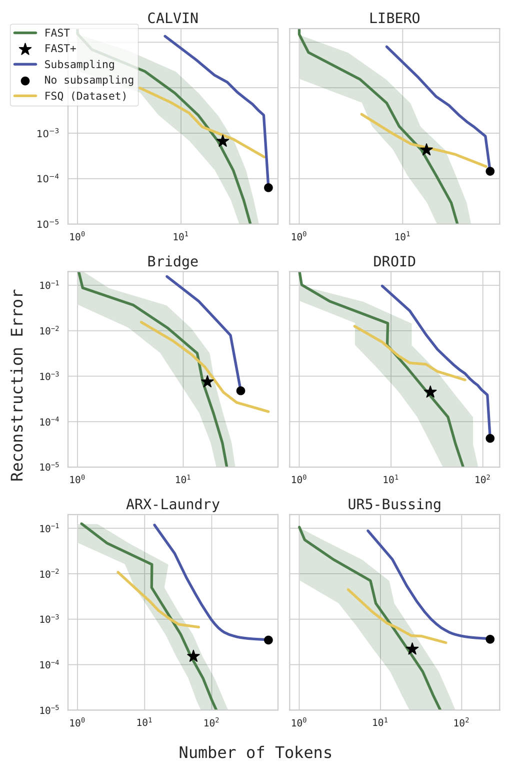
Reading the figure: Learned FSQ can be effective at low precision and very few tokens. At higher precision, FAST's error decreases more with token count and better suits the tested fine-control tasks. The shortest sequence is not automatically the best trajectory representation.

Limits: Very small quantization scales can erase coefficients and produce near-constant motion; large scales improve fidelity but create fewer compressible zeros and more complex integers. Larger vocabularies represent more combinations but consume more output slots. The tested range does not establish monotonic performance gains.

Engineering note: Predicted tokens or expanded lengths can be invalid. Check chunk shape, effective dimensions, and control limits before execution. v1 does not fully specify repairs, so padding or truncation must not be presented as a documented paper implementation.

The Complete π0-FAST Network

Inputs and Shapes

Each prediction conditions on:

• Two or three RGB images of $224\times224\times3$.

• Natural-language instruction $\ell_t$.

• Proprioception $q_t$, with platform-dependent dimensions.

• During training only, real future actions $A_t\in\mathbb R^{H\times D}$ for FAST supervision.

Table I's shirt setting uses $H=50,D=14$, giving $50\times14$ labels; its DROID setting uses $H=15,D=7$, giving $15\times7$. Use the effective action space for the actual dataset version.

Difference from π0: π0 continuously projects state and noisy actions into an expert. FAST v1 bins current state into 256 levels and tokenizes the integers as text, while future actions use FAST. State is a current condition rather than a long high-rate output, so the authors consider simple binning sufficient there.

Image and Text Features in One Backbone

A pre-trained encoder produces visual tokens per camera; task and state strings produce text tokens. Together they form the observation prefix. PaliGemma-3B is the main backbone, with OpenVLA/Prismatic 7B as a transfer comparison.

Explanation: With $N_v$ tokens per image and $N_\ell,N_q$ language/state tokens, prefix length is:

$N_o=mN_v+N_\ell+N_q$

$m$ is camera count and $N_o$ prefix length, ignoring a few separators/special tokens. For embedding width $E$, the representation is $N_o\times E$. This explains dimensions, not a complete v1 specification; visual counts, width, separators, and position encodings are not all given.

Action Suffix and Attention

FAST encodes demonstrated actions as $n$ tokens, mapped to rarely used VLM slots and supplied as a prediction suffix after the observation prefix.

Explanation: Predicting token $k$ uses observations and the preceding $k-1$ action tokens, never future labels. This is causal autoregression, with no CVAE encoder or continuous-flow decoder.

The backbone's hidden states become vocabulary logits and classification probabilities. $V=1024$ is the action vocabulary in dataset-specific experiments, not the full language vocabulary.

Policy Training Loss

Explanation: Standard negative log-likelihood expresses the stated next-token objective:

$\mathcal L_{\rm AR}(\theta) =\mathbb E_{(o_t,A_t)}\left[ -\sum_{k=1}^{n}\log p_\theta(z_k\mid o_t,z_{<k}) \right],\qquad z_{1:n}=\mathcal T(A_t)$

$\mathcal L_{\rm AR}$ is autoregressive loss, $\theta$ policy weights, and expectation averages demonstrations; $n$ varies by sample. v1 does not fully specify token averaging or treatment of end symbols.

Teacher forcing uses ground-truth $z_{<k}$ during training. A causal mask allows losses at all positions in one forward pass, while inference depends on generated prefixes and proceeds sequentially. Shorter targets reduce overhead without removing inference's serial dependence.

Paper configuration: 1,000 linear warmup steps, then learning rate $5\times10^{-5}$; AdamW with $\beta_1=0.9,\beta_2=0.95$, no weight decay, gradient clipping at 1, and exponential moving average coefficient 0.999. All policy weights are fine-tuned.

Sampling and Continuous Outputs

Most tasks use greedy decoding. Bimanual shirt folding, toast removal, and laundry use temperature 0.7, which the authors find helps escape near-stationary behavior around initial poses.

Explanation: For logits $r_{k,v}$ and temperature $\eta>0$:

$p_{k,v}=\frac{\exp(r_{k,v}/\eta)}{\sum_{w}\exp(r_{k,w}/\eta)}$

$v,w$ index candidates and $p_{k,v}$ is sampling probability. The guide uses $\eta$ to distinguish temperature from optimizer $\beta_1,\beta_2$; the paper writes temperature $\beta=0.7$. It differs from quantization scale $\gamma=10$.

FAST decodes tokens to $\widehat A_t\in\mathbb R^{H\times D}$ in the dataset's physical units. DROID uses joint velocity and absolute gripper position; other tasks use their platform settings. Controllers execute valid actions, then new observations generate the next chunk.

Ablation: After adding multi-image input and one-second chunks to OpenVLA, replacing binning with FAST+ substantially improves shirt folding. Benefits extend beyond the π0 backbone, but the test does not establish equal gains for every VLM.

Complete Flow Compared with π0

Training:
Demonstration images + task language + current state + real next-second actions
→ Encode images as visual tokens
→ Tokenize language and discretized state text as the observation prefix
→ Normalize actions; DCT; quantize; frequency-first flatten; BPE
→ Map action tokens to VLM output slots
→ Compute teacher-forced next-token cross-entropy
→ Fine-tune all policy weights to obtain π0-FAST

Inference:
Current images + task language + state
→ Construct observation prefix
→ Greedily decode or sample action tokens at the specified temperature
→ Reverse BPE and restore integer coefficient ordering
→ Dequantize, inverse DCT, denormalize
→ Obtain an H × D continuous chunk
→ Execute the configured steps with the low-level controller
→ Observe and predict again

In one sentence:
The VLM selects actions from the scene and task;
DCT concentrates shared information from densely sampled trajectories;
quantization and BPE turn coefficients into shorter token sequences;
autoregressive training models their conditional distribution, and FAST decoding restores continuous control.
The main benefits are action representation and training efficiency; v1 inference latency remains a major limitation.