Stage 5 · Chapter 24 · Theory

24. Forward Kinematics, Inverse Kinematics, and the Jacobian

Chapter 24 of the Seeed Physical AI Beginner's Course — joint space versus Cartesian space, forward kinematics from DH parameters and URDF, inverse kinematics and its multiple or missing solutions, the Jacobian and velocity kinematics, singularities and damped least squares, and analytic versus numerical IK.

Joint vs CartesianForward kinematicsInverse kinematicsJacobian

24.1 Main Topics

• Joint space vs. Cartesian space
• Forward kinematics (FK)
• Inverse kinematics (IK)
• Multiple solutions, no solution, and workspace
• Joint limits
• Jacobian matrix
• Velocity kinematics
• Singularities
• Numerical IK and closed-loop IK

24.2 Learning Objectives

Explain how the arm computes the end-effector pose from joint angles, and how to solve for joint angles given a target pose.

24.3 Joint Space vs. Cartesian Space

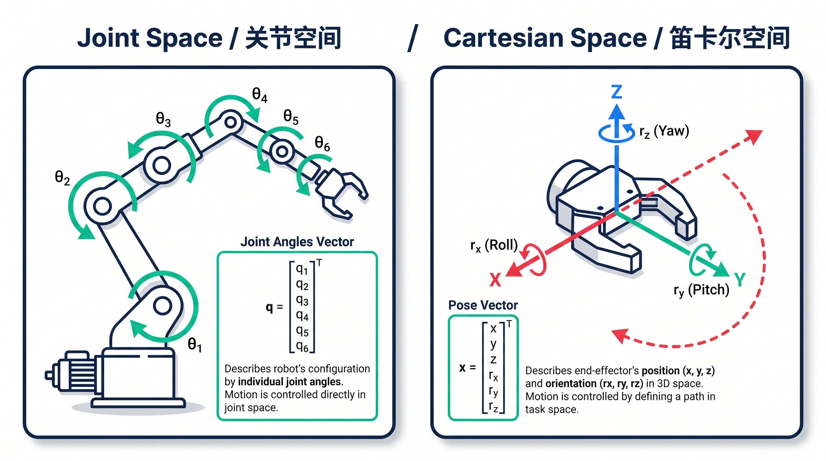
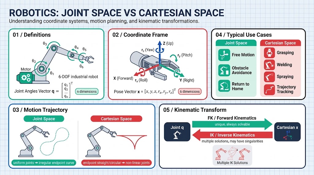
	Joint Space	Cartesian Space
Description	Joint angles $(q_1, q_2, \ldots, q_n)$	End-effector pose $(x, y, z, rx, ry, rz)$
Dimension	n (number of joints)	6 (3 position + 3 orientation)
Physical meaning	How the motors turn	Where the end is and which way it faces
Motion path	Constant joint velocity -> irregular end-effector curve	Straight/arc end path -> nonlinear joint motion
Control difficulty	Direct (send to motors)	Indirect (must solve IK for joint angles first, then send to motors)
Typical uses	Free motion, obstacle avoidance, homing	Grasping, welding, painting, path following

Example 1: writing robot

Task	Which space
Turn motor 1 by 30 deg, motor 2 by 45 deg	Joint space (send angles directly)
Make the pen tip trace the strokes of a character in straight lines	Cartesian space (compute joint angles for each point)

Example 2: picking up a cup (ignoring the path)

Stage	Which space
Move from home to near the cup	Joint space (simple, constant speed, safe)
Final few centimeters to precisely align with the cup rim	Cartesian space (must approach in XYZ)
Lift and place on the shelf	Joint space (no straight-line requirement)

Example 3: welding a car

Task	Which space
Welding torch follows the seam in a straight line	Cartesian space (straight line = weld seam)
Lift the torch and move to the next spot	Joint space (fast is what matters)

24.4 Forward vs. Inverse Kinematics

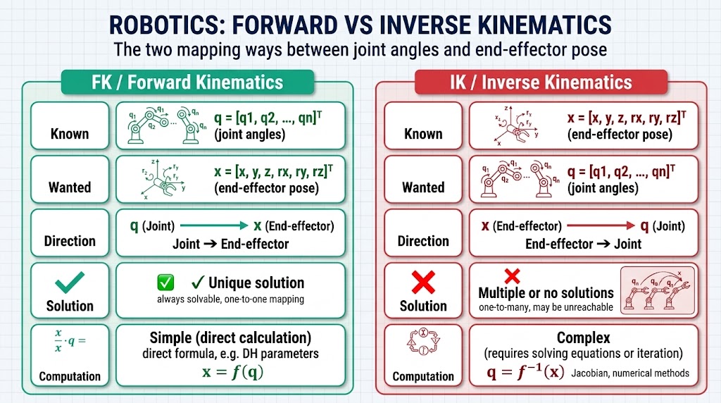
	Forward Kinematics (FK)	Inverse Kinematics (IK)
Known	Joint angles	End-effector pose
Solve for	End-effector pose	Joint angles
Direction	Joints -> end-effector	End-effector -> joints
Solution	Unique	Multiple / none
Computation	Simple (apply formulas directly)	Complex (solve equations / iterate)

What FK is used for

• Visualization: render joint angles live as a 3D model (ROS RViz, game characters)
• Verification: check whether the computed end-effector pose is correct
• Calibration: compare theoretical pose with actual pose
• Simple control: move along a preset angle sequence

What IK is used for

• Grasping: camera sees object -> solve joint angles -> control the arm
• Welding/painting: end must follow a specified trajectory
• Humanoid: feet must land on specified ground points
• Any "go to a place" scenario

24.5 Forward Kinematics

The process of computing the end-effector pose from joint angles

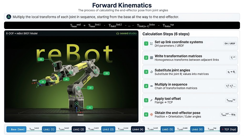
One-sentence version

Multiply the local transform of each joint in sequence, from the base all the way to the end-effector.

$$T_{base}^{end} = T_{base}^{link_1} \cdot T_{link_1}^{link_2} \cdots T_{link_{n-1}}^{link_n} \cdot T_{link_n}^{tcp}$$

Computation steps (6 steps)

1. Establish link frames: build a local frame at each joint (DH parameters / URDF)
2. Write each link's transform matrix $T_i^{i+1}$ (translation + rotation relative to the previous joint)
3. Substitute joint angles $q_i$ (rotation uses $\theta_i$, translation comes from the DH table)
4. Multiply in sequence $T_1^2 \cdot T_2^3 \cdot \ldots \cdot T_n^{n+1}$
5. Multiply by the tool offset $T_{flange}^{tcp}$
6. Obtain $T_{base}^{end}$ — containing position $(x,y,z)$ and orientation ($R$ or $q$ or Euler angles)

Related concepts in one diagram

Joint angles (q)
   |
DH params / URDF  ← describe link geometry (a, alpha, d, theta)
   |
Homogeneous transform (4x4)  ← translation + rotation combined
   |
   +-- rotation matrix R (3x3, SO(3))
   |      +-- rotation representation: Euler / quaternion / axis-angle
   +-- translation vector t (3x1)
   |
Matrix chain multiplication (chain rule)
   |
End-effector pose T_base^end (SE(3))
   |
   +-- position (x, y, z)  ← FK output
   +-- orientation (R / q / rpy)  ← orientation representation
   |
Cartesian-space trajectory / Jacobian (velocity mapping)
   |
Visualization (RViz / simulation)

Core concept checklist

Concept	Role
DH parameters	Encode each link's $a, \alpha, d, \theta$ as 4 numbers
Homogeneous transform	Pack translation + rotation into a 4x4 matrix for easy chaining
Chain rule	The essence of multiplying many matrices
Rotation representation	Output orientation as: Euler angles / quaternion / rotation matrix
Trigonometry	Matrix expansion is all $\sin/\cos$
Jacobian	FK gives pose; J gives velocity (used in reverse by IK)
URDF	The actual robot description file; source of FK numbers

A small example (2 joints)

$$\theta_1, \theta_2 = \text{joint angles}, \qquad l_1, l_2 = \text{link lengths}$$$$T_1^2 = \begin{pmatrix} \cos\theta_1 & -\sin\theta_1 & 0 & l_1\cos\theta_1 \\ \sin\theta_1 & \cos\theta_1 & 0 & l_1\sin\theta_1 \\ 0 & 0 & 1 & 0 \\ 0 & 0 & 0 & 1 \end{pmatrix} \qquad T_2^3 = \begin{pmatrix} \cos\theta_2 & -\sin\theta_2 & 0 & l_2\cos\theta_2 \\ \sin\theta_2 & \cos\theta_2 & 0 & l_2\sin\theta_2 \\ \vdots & \vdots & \vdots & \vdots \\ 0 & 0 & 0 & 1 \end{pmatrix}$$$$T_1^3 = T_1^2 \, T_2^3 \quad\Longrightarrow\quad \text{end-effector pose}$$

FK = DH description + homogeneous matrices + chain multiplication, translating "joint angles" into "where the end is."

Must-know along the way: DH, 4x4 transforms, matrix multiplication, rotation representations (Euler/quaternion), URDF.

24.6 Inverse Kinematics

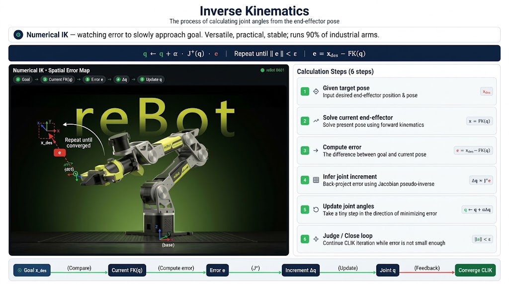
The process of computing joint angles from the end-effector pose. In practice it is almost always done numerically: instead of solving the pose equation in one step, the solver approaches the target gradually.

Think of reaching for a book on a shelf: you look at how far your hand still is from the book, decide which way to move, shift your joints a little, and repeat until you touch it. A robot does exactly the same thing.

The loop — each iteration does three things:

1. Look at the error: how far the end-effector still is from the target pose
2. Infer the direction: how each joint must move to reduce that error
3. Take a step: move the joints once, then go back to step 1

Repeat until the error is small enough.

Why it is used so widely

• Universal: the same loop works for 6-axis, 7-axis, hands and snake arms
• No formulas to derive: it is a program, not a page of algebra
• Adjustable precision: want more accuracy? Run more iterations

In industry the loop is closed around the measured joint positions, so the controller keeps watching the error and correcting even when the model is slightly wrong. This "look while moving" version is CLIK (Closed-Loop IK), the de facto standard on factory arms.

In one sentence: numerical IK = watch the error and approach the target little by little — universal, effective and stable.

24.7 Jacobian Matrix

The Jacobian turns "solving for pose" into "solving for velocity".

The pose equation is nonlinear and usually has no closed-form solution:

$$f(q) = T_{target}$$

Differentiating it at the current $q$ gives the Jacobian, and to first order the problem becomes linear:

$$J(q) = \frac{\partial f}{\partial q}, \qquad v_{end} = J(q)\,\dot{q}, \qquad \Delta T \approx J(q)\,\Delta q, \qquad \dot{q} = J^{-1} v_{end}$$

The iterative loop

1. Current $q$ -> compute the end-effector pose $T$
2. Error: $\Delta T = T_{target} - T$
3. End-effector velocity: $v = \Delta T / dt$
4. Joint velocity: $\dot{q} = J^{-1} v$
5. Update: $q_{new} = q + \dot{q}\,dt$
6. Back to 1, until $\Delta T$ is small enough

In one sentence: the Jacobian "locally flattens" the nonlinear IK equation into a linear one; solving for the velocity and integrating it converges to the target pose.

24.8 Singularities

At a singularity the arm loses the ability to move the end-effector in one or more directions — no matter how the joints move, the end cannot move that way.

• Arm fully extended: it cannot reach any further out; the outward direction is lost
• Two wrist joints collinear: two rotation axes coincide, so one degree of freedom disappears

What happens at a singularity

Situation	Symptom
Jacobian "fails"	The joint-to-end mapping can no longer be inverted
IK solution explodes	Computed joint velocity goes to infinity
Joint twitching	Motors shake violently
Control oscillation	The end jumps back and forth

Essence: some entries of that mapping become $0/0$ — undefined, not merely large.

How to detect it — when the Jacobian degenerates, one number goes to zero:

$$\det J = 0, \qquad \sigma_{\min}(J) = 0, \qquad \operatorname{rank} J < n$$

Monitor that number and raise an alarm as it approaches zero.

How to handle it

Fix	Idea
Damped least squares (DLS)	Add some "friction" so the solution cannot explode: $\dot{q} = J^\top (J J^\top + \lambda^2 I)^{-1} v$
Change the path	Plan ahead to bypass singular regions
Slow down	Decelerate near a singularity to give yourself reaction time
Change the pose	For the same target pose, pick a non-singular solution

Two kinds of singularities

• Workspace boundary: extended to the farthest point; directions are lost
• Workspace interior: wrist collinear / elbow straight; degrees of freedom are reduced

24.9 Analytic IK vs. Numerical IK

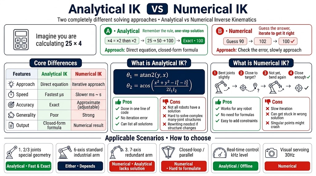
Analytic IK solves the equation directly; numerical IK iterates towards the answer. The same task — computing $25 \times 4$ — done both ways:

	Analytic	Numerical
Idea	"×4 means ×2 then ×2": work out $25 \times 2 = 50$, then $\times 2 = 100$	Guess 90, notice it is 10 short, guess 102, then 100 — adjust until it matches
Result	One step, exact	A few iterations, close enough

Core differences

Dimension	Analytic IK	Numerical IK
Approach	Directly solve the equation	Iterative approximation
Speed	Fastest (microseconds)	Slower (ms~s)
Accuracy	Exact	Approximate (adjustable)
Generality	Poor	Strong
Output	Closed-form formula	Numerical result

Analytic IK — solve the equation once and for all, and you get formulas such as

$$\theta_1 = \operatorname{atan2}(\ldots), \qquad \theta_2 = \operatorname{acos}(\ldots), \qquad \vdots$$

Pros	Cons
Computed in one line of code; no iteration error; can list all solutions	Not every robot has a closed-form solution; with many joints and a complex structure the equation cannot be solved; once the robot changes, every formula must be rewritten

Numerical IK — no formula at all, just repeat "bend the joints a little, check whether the end got closer, if not bend a bit more" until it is close enough.

Pros	Cons
Works for any robot; no equations to derive; easy to add constraints	Slow (needs iteration); may get stuck at a wrong solution; explodes at singularities

Applicable scenarios

Scenario	Choose
2-joint, 3-joint, special geometry	Analytic (fast, exact)
6-axis standard industrial arm	Either, depends on scenario
7-axis redundant arm	Numerical (no analytic solution)
Closed-loop / parallel	Numerical (analytic is hard to derive)
Real-time control (kHz)	Analytic or offline-generated analytic solution
Visual servoing (30 Hz)	Numerical

Key takeaways

• Joint space is what the motors understand; Cartesian space is what the task understands.
• FK is unique, cheap and always solvable; IK may have several solutions, one solution, or none.
• The Jacobian converts joint velocity into end-effector velocity, and is how IK is actually solved.
• Singularities are poses where the Jacobian loses rank; detect them (smallest singular value) and damp them (DLS).
• Next chapter: once you can produce a pose, you still have to move there smoothly and safely.