Few-Shot Object Detection with YOLOv5 and Roboflow

Introduction

YOLO is one of the most famous object detection algorithms available. It only needs few samples for training, while providing faster training times and high accuracy. We will demonstrate these features one-by-one in this wiki, while explaining the complete machine learning pipeline step-by-step where you collect data, label them, train them and finally detect objects using the trained data by running the trained model on an edge device such as the NVIDIA Jetson platform. Also, we will compare the difference between using custom datasets and public datasets.

What is YOLOv5?

YOLO is an abbreviation for the term ‘You Only Look Once’. It is an algorithm that detects and recognizes various objects in an image in real-time. Ultralytics YOLOv5 is the latest version of YOLO and it is now based on the PyTorch framework.

What is few-shot object detection?

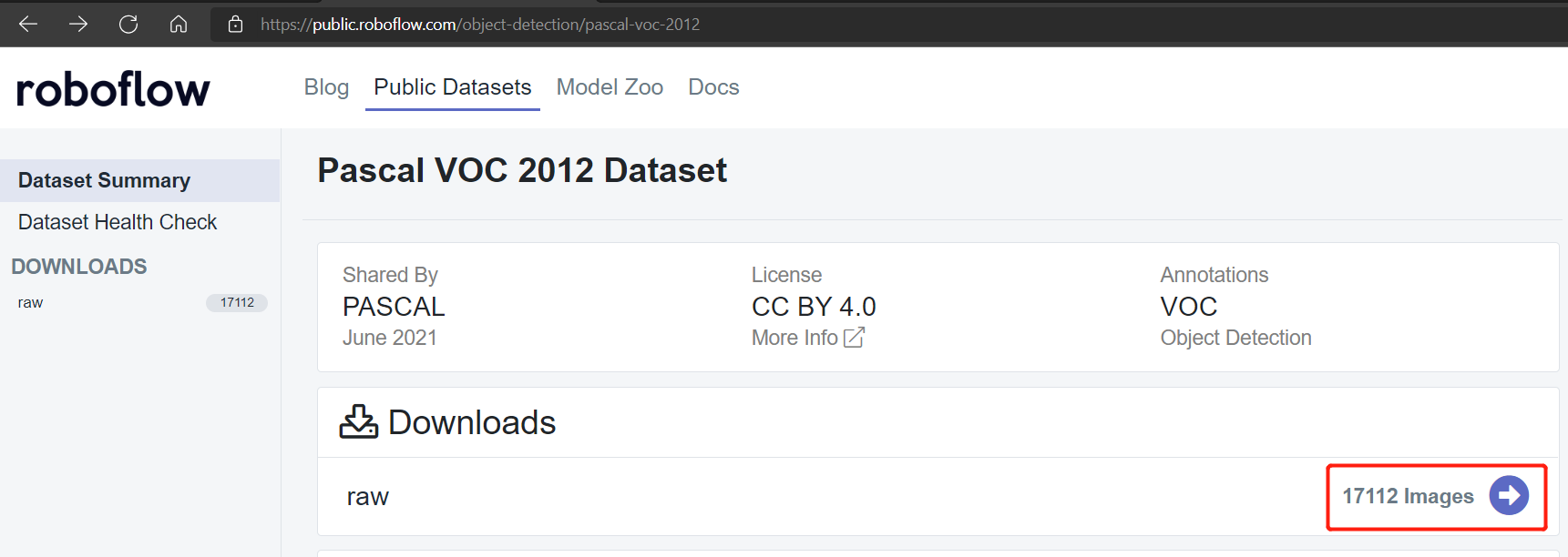
Traditionally if you want to train a machine learning model, you would use a public dataset such as the Pascal VOC 2012 dataset which consists of around 17112 images. However, we will use transfer learning to realize few-shot object detection with YOLOv5 which needs only a very few training samples. We will demonstate this in this wiki.

Hardware supported

YOLOv5 is supported by the following hardware:

• Official Development Kits by NVIDIA:

  • NVIDIA® Jetson Nano Developer Kit
  • NVIDIA® Jetson Xavier NX Developer Kit
  • NVIDIA® Jetson AGX Xavier Developer Kit
  • NVIDIA® Jetson TX2 Developer Kit

• Official SoMs by NVIDIA:

  • NVIDIA® Jetson Nano module
  • NVIDIA® Jetson Xavier NX module
  • NVIDIA® Jetson TX2 NX module
  • NVIDIA® Jetson TX2 module
  • NVIDIA® Jetson AGX Xavier module

• Carrier Boards by Seeed:

  • Jetson Mate
  • Jetson SUB Mini PC
  • Jetson Xavier AGX H01 Kit
  • A203 Carrier Board
  • A203 (Version 2) Carrier Board
  • A205 Carrier Board
  • A206 Carrier Board

Prerequisites

• Any of the above Jetson devices running latest JetPack v4.6.1 with all SDK components installed (check this wiki for a reference on installation)

• Host PC

  • Local training needs a Linux PC (preferably Ubuntu)
  • Cloud training can be performed from a PC with any OS

Getting started

Running your first object detection project on an edge device such as the Jetson platform simply involves 4 main steps!

1. Collect dataset or use publically available dataset

   • Collect dataset manually
   • Use publicly available dataset

2. Annotate dataset using Roboflow

3. Train on local PC or cloud

   • Train on local PC (Linux)
   • Train on Google Colab

4. Inference on Jetson device

Collect dataset or use publically available dataset

The very first step of an object detection project is to obtain data for training. You can either download datasets available publicly or create your own dataset! Usually public datasets are used for education and research purposes. However, if you want to build specific object detection projects where the public datasets do not have the objects that you want to detect, you might want to build your own dataset.

Collect dataset manually

It is recommended that you first record a video footage of the object that you want to recognize. You have to make sure that you cover all angles (360 degrees) of the object, place the object in different environments, different lighting and different weather conditions. The total video we recorded is 9 minutes long where 4.5 minutes is for flowers and the remaining 4.5 minutes is for leaves. The recording can be broken down as follows:

1. morning normal weather
2. morning windy weather
3. Morning rainy weather
4. Noon normal weather
5. Noon windy weather
6. Noon rainy weather
7. Evening normal weather
8. Evening windy weather
9. Evening rainy weather

Note: Later on, we will convert this video footage into a series of images to make up the dataset for training.

Use publicly available dataset

You can download a number of publically available datasets such as the COCO dataset, Pascal VOC dataset and much more. Roboflow Universe is a recommended platform which provides a wide-range of datasets and it has 90,000+ datasets with 66+ million images available for building computer vision models. Also, you can simply search open-source datasets on Google and choose from a variety of datasets available.

Annotate dataset using Roboflow

Next we will move on to annotating the dataset that we have. Annotating means simply drawing rectangular boxes around each object that we want to detect and assign them labels. We will explain how to do this using Roboflow.

Roboflow is an annotation tool based online. Here we can directly import the video footage that we recorded before into Roboflow and it will be exported into a series of images. This tool is very convenient because it will let us help distribute the dataset into "training, validation and testing". Also this tool will allow us to add further processing to these images after labelling them. Furthermore, it can easily export the labelled dataset into YOLOV5 PyTorch format which is what we exactly need!

• Step 1. Click here to sign up for a Roboflow account

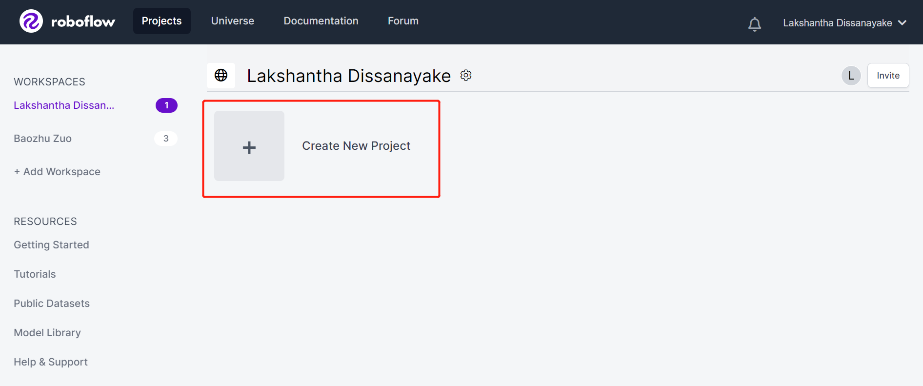
• Step 2. Click Create New Project to start our project

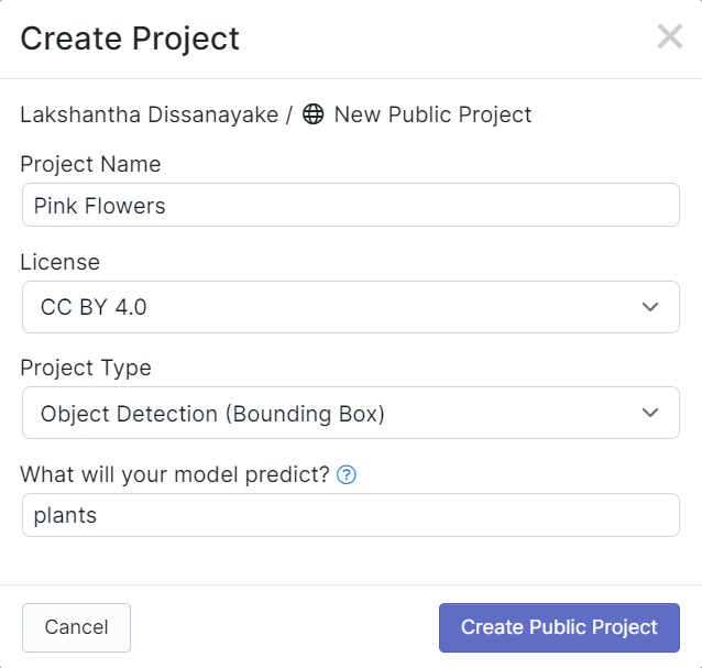
• Step 3. Fill in Project Name, keep the License (CC BY 4.0) and Project type (Object Detection (Bounding Box)) as default. Under What will your model predict? column, fill in an annotation group name. For example, in our case we choose plants. This name should highlight all of the classes of your dataset. Finally, click Create Public Project.

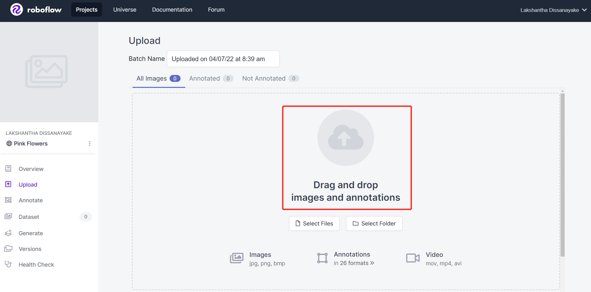
• Step 4. Drag and drop the video footage that you recorded before

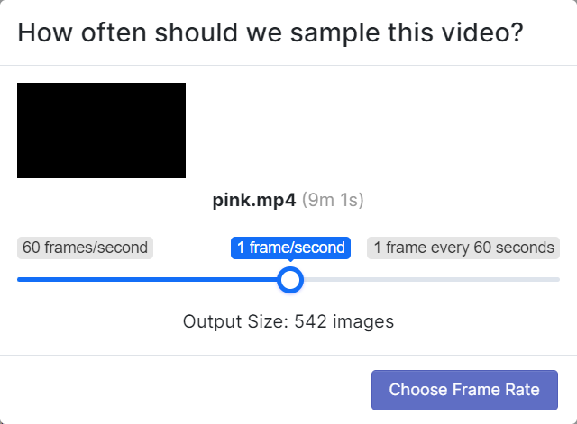
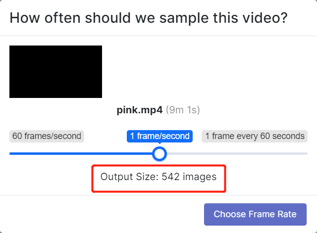
• Step 5. Choose a framerate so that the video will be divided into a series of images. Here we will use the default frame rate which is 1 frame/second and this will generate 542 images in total. Once you select a frame rate by scrubbing through the slider, click Choose Frame Rate. It will take a few seconds to a few minutes (depending on the video length) to finish this process.

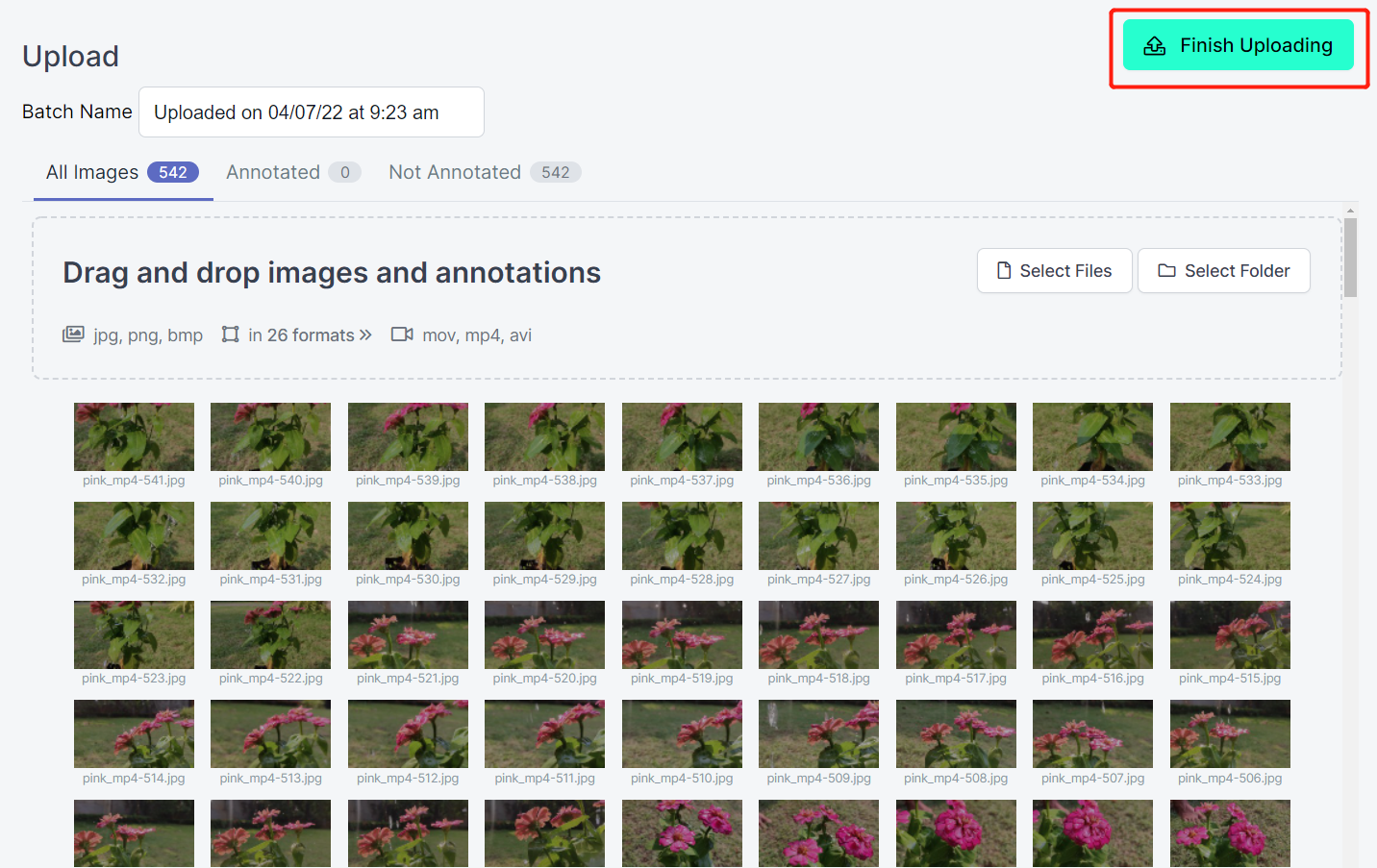
• Step 6. After the images are processed, click Finish Uploading. Wait patiently until the images are uploaded.

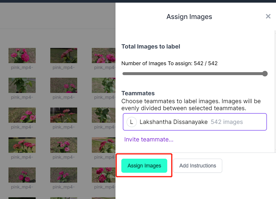
• Step 7. After the images are uploaded, click Assign Images

• Step 8. Select an image, draw a rectangular box around a flower, choose the label as pink flower and press ENTER

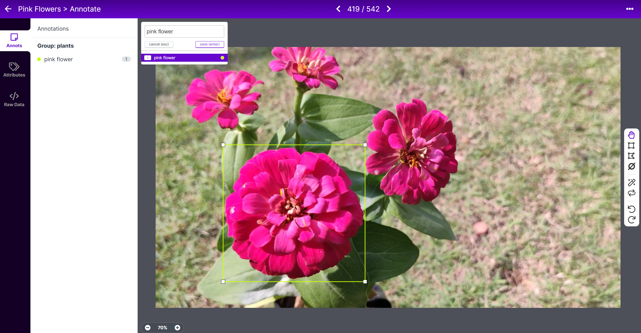
• Step 9. Repeat the same for the remaining flowers

• Step 10. Draw a rectangular box around a leaf, choose the label as leaf and press ENTER

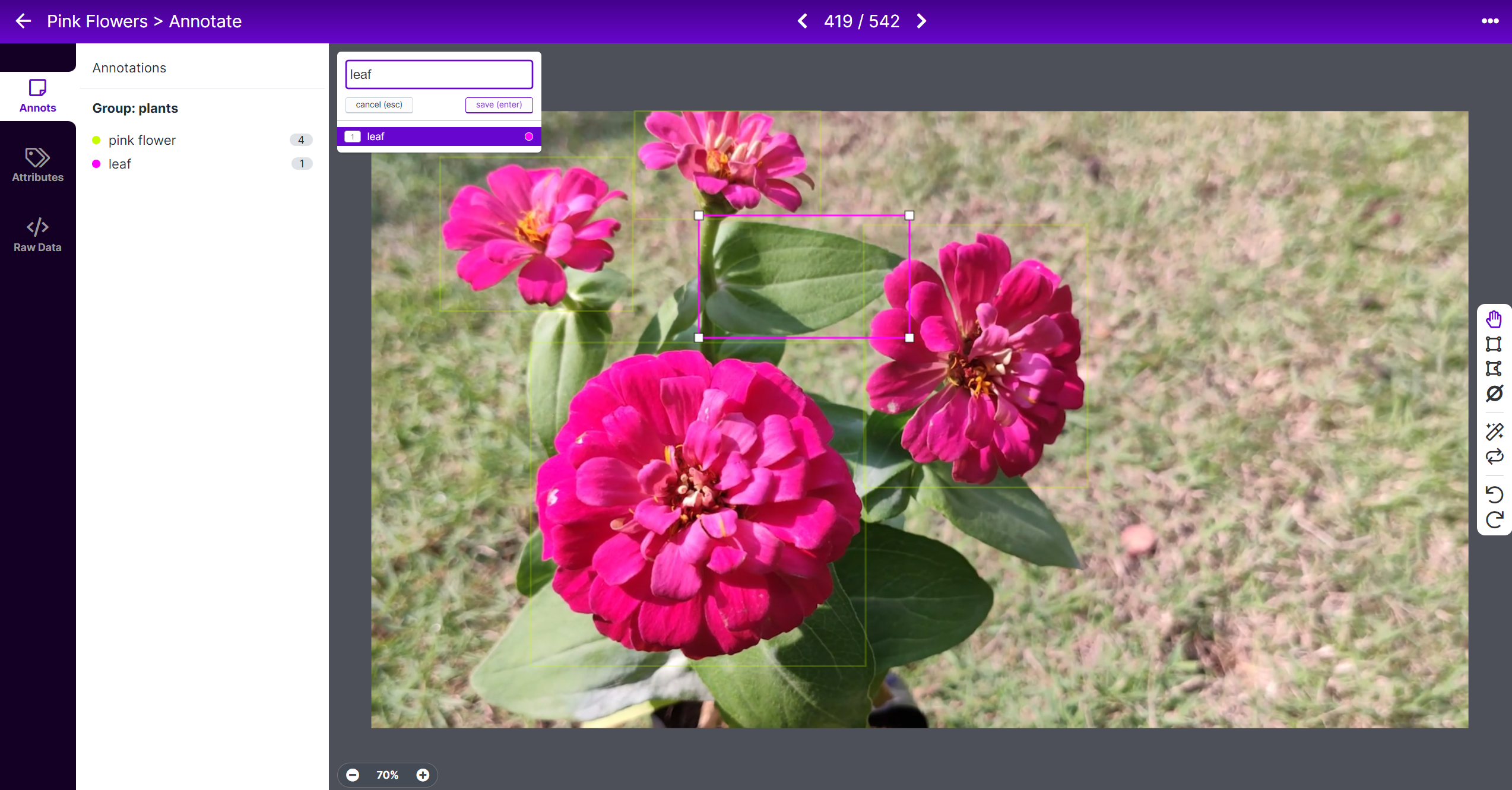
• Step 11. Repeat the same for the remaining leaves

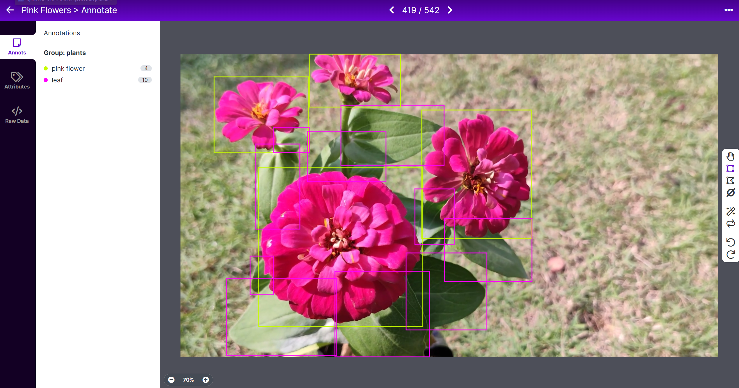
Note: Try to label all the objects that you see inside the image. If only a part of the object is visible, try to label that too.

• Step 12. Continue to annotate all the images in the dataset

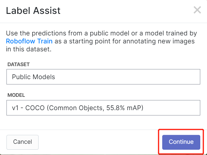
Roboflow has a feature called Label Assist where it can predict the labels beforehand so that your labelling will be much faster. However, it will not work with all object types, but rather a selected type of objects. To turn this feature on, you simply need to press the Label Assist button, select a model, select the classes and navigate through the images to see the predicted labels with bounding boxes

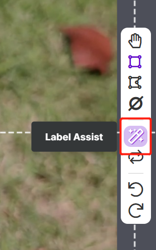
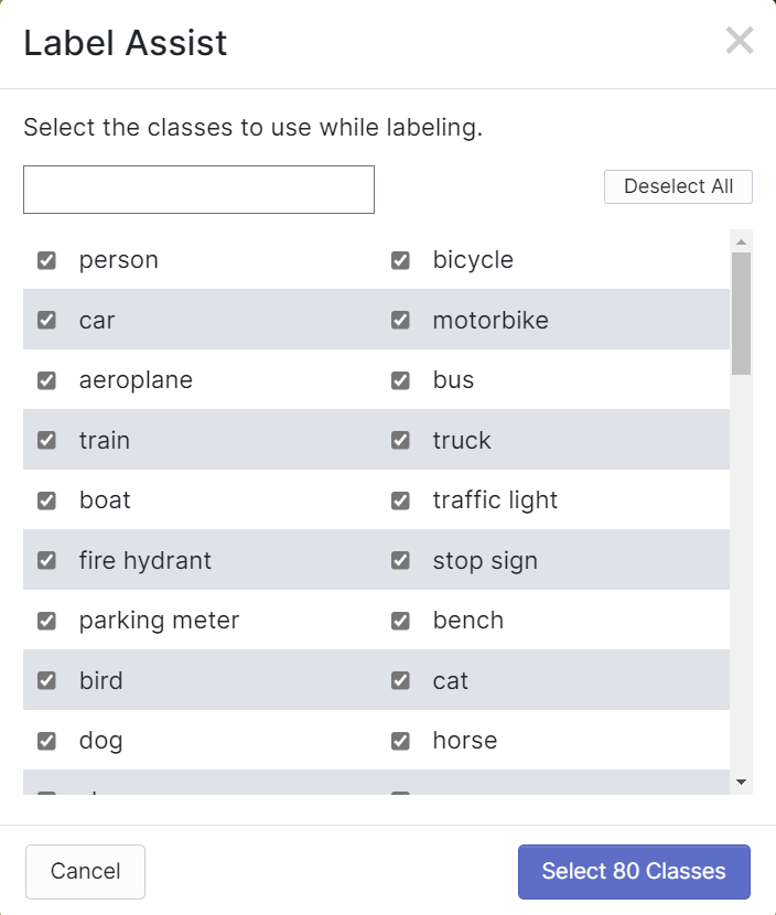
As you can see above, it can only help to predict annotations for the 80 classes mentioned. If your images do not contain the object classes from above, you cannot use the label assist feature.

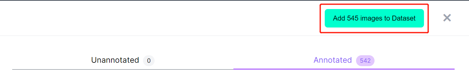
• Step 13. Once labelling is done, click Add images to Dataset

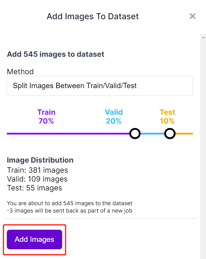
• Step 14. Next we will split the images between "Train, Valid and Test". Keep the default percentages for the distribution and click Add Images

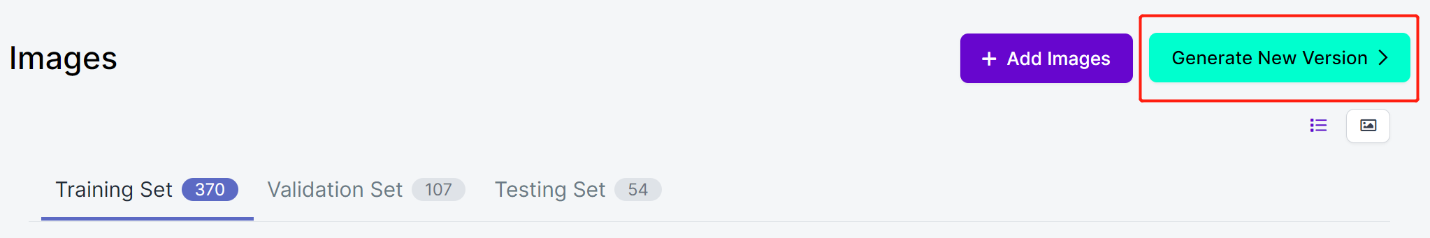
• Step 15. Click Generate New Version

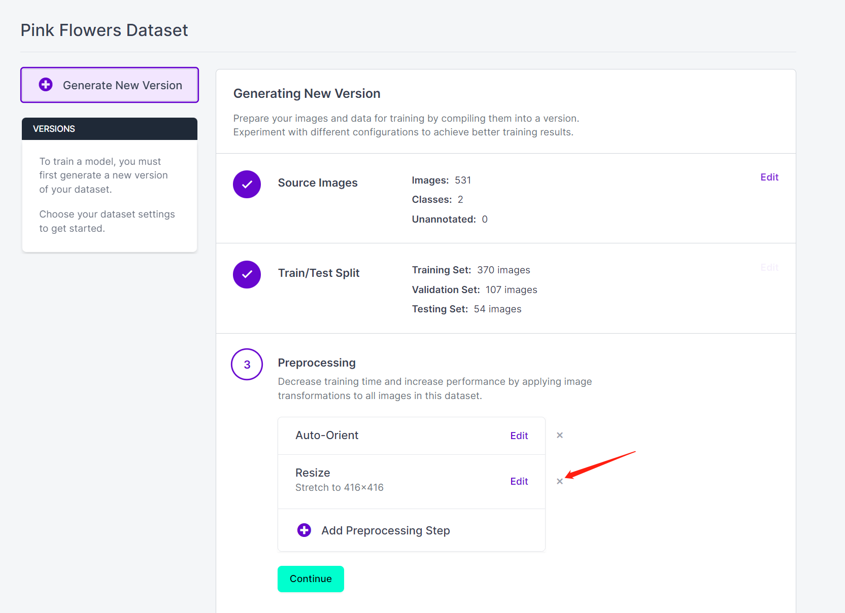
• Step 16. Now you can add Preprocessing and Augmentation if you prefer. Here we will delete the Resize option and keep the original image sizes

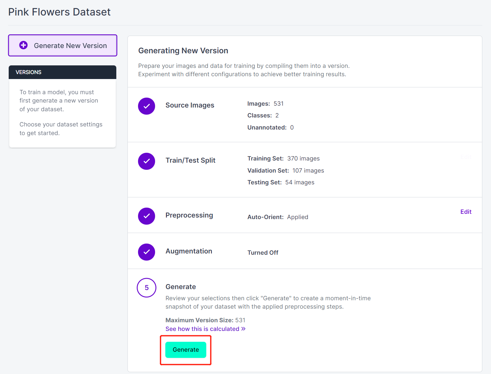
• Step 17. Next, proceed with the remaining defaults and click Generate

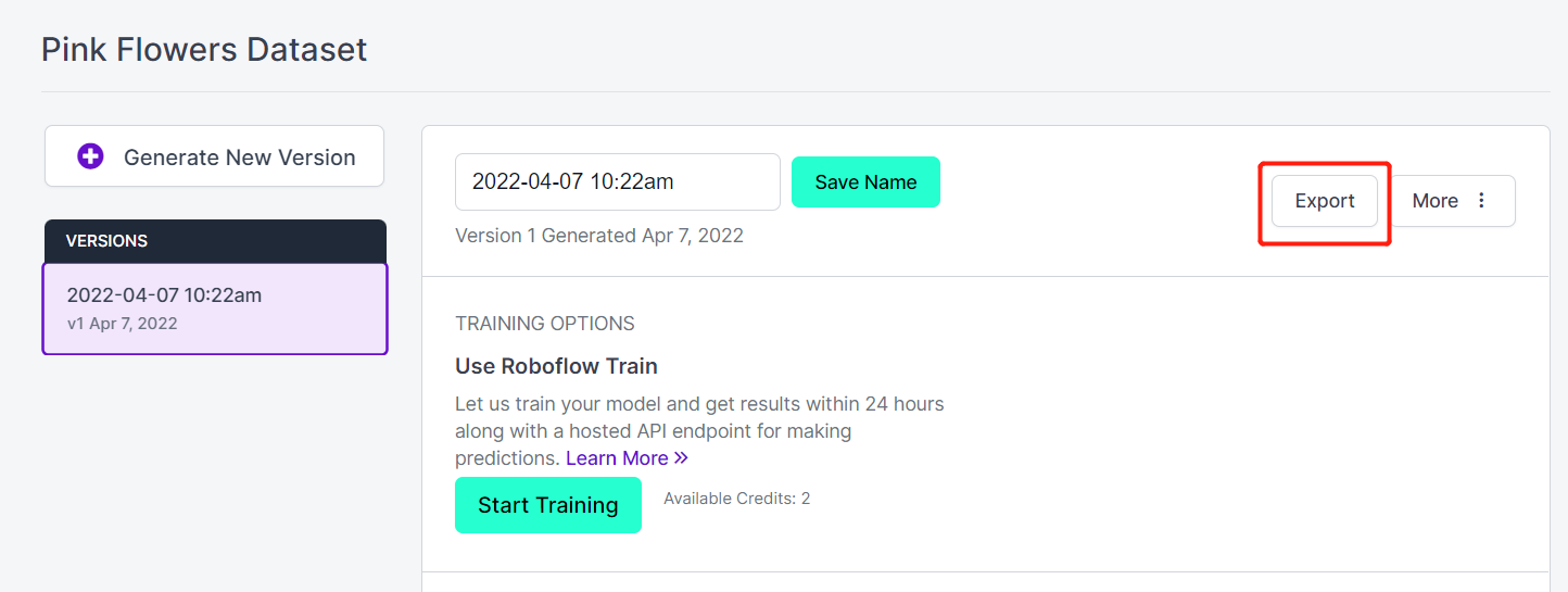
• Step 18. Click Export

• Step 19. Select download zip to computer, under "Select a Format" choose YOLO v5 PyTorch and click Continue

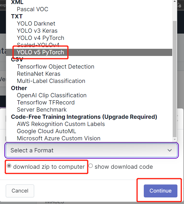
• Step 20. After that, a .zip file will be downloaded to your computer. We will need this .zip file later for our training.

Train on local PC or cloud

After we are done with annotating the dataset, we need to train the dataset. For training we will introduce two methods. One method will be based online (Google Colab) and the other method will be based on local PC (Linux).

For the Google Colab training, we will use two methods. In the first method, we will use Ultralytics HUB to upload the dataset, setup training on Colab, monitor the training and grab the trained model. In the second method, we will grab the dataset from Roboflow via Roboflow api, train and download the model from Colab.

Use Google Colab with Ultralytics HUB

Ultralytics HUB is a platform where you can train your models without having to know a single line of code. Simply upload your data to Ultralytics HUB, train your model and deploy it into the real world! It is fast, simple and easy to use. Anyone can get started!

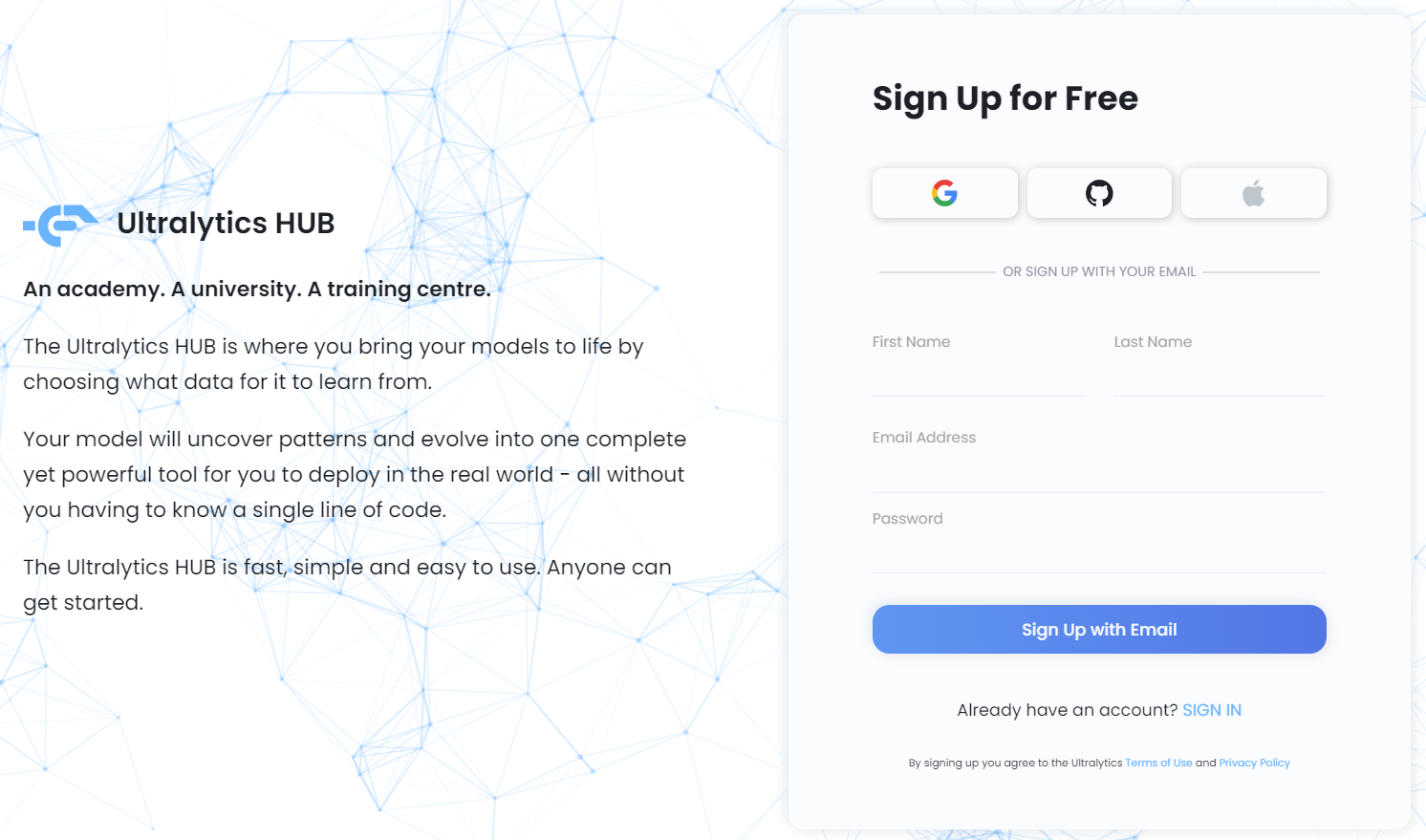
• Step 1. Visit this link to sign up for a free Ultralytics HUB account

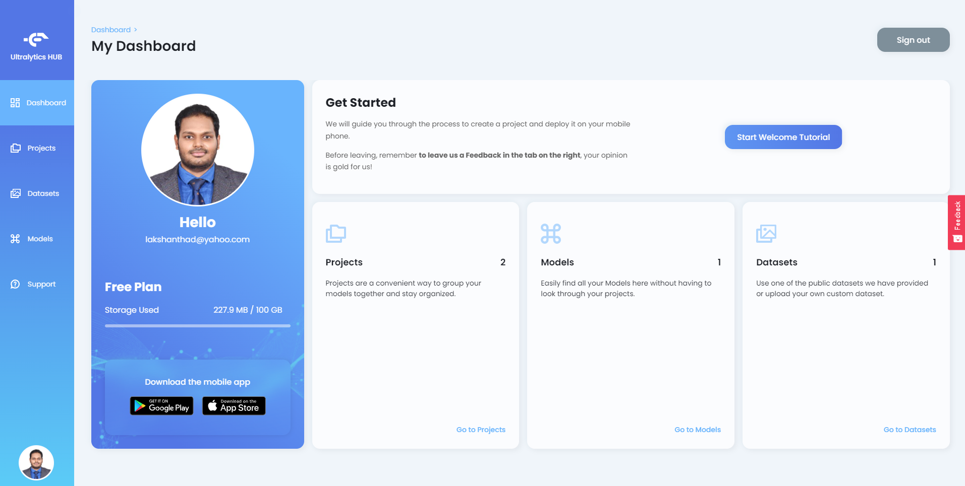
• Step 2. Enter your credentials and sign up with email or sign up directly with a Google, GitHub or Apple account

After you login to Ultralytics HUB, you will see the dashboard as follows

• Step 3. Extract the zip file that we downloaded before from Roboflow and put all the included files inside a new folder

• Step 4. Make sure your dataset yaml and root folder (the folder we created before) share the same name. For example, if you name your yaml file as pinkflowers.yaml, the root folder should be named as pinkflowers.

• Step 5. Open pinkflowers.yaml file and edit train and val directories as follows

train: train/images
val: valid/images

• Step 6. Compress the root folder as a .zip and name it the same as the root folder (pinkflowers.zip in this example)

Now we have prepared the dataset which is ready to be uploaded to Ultalytics HUB.

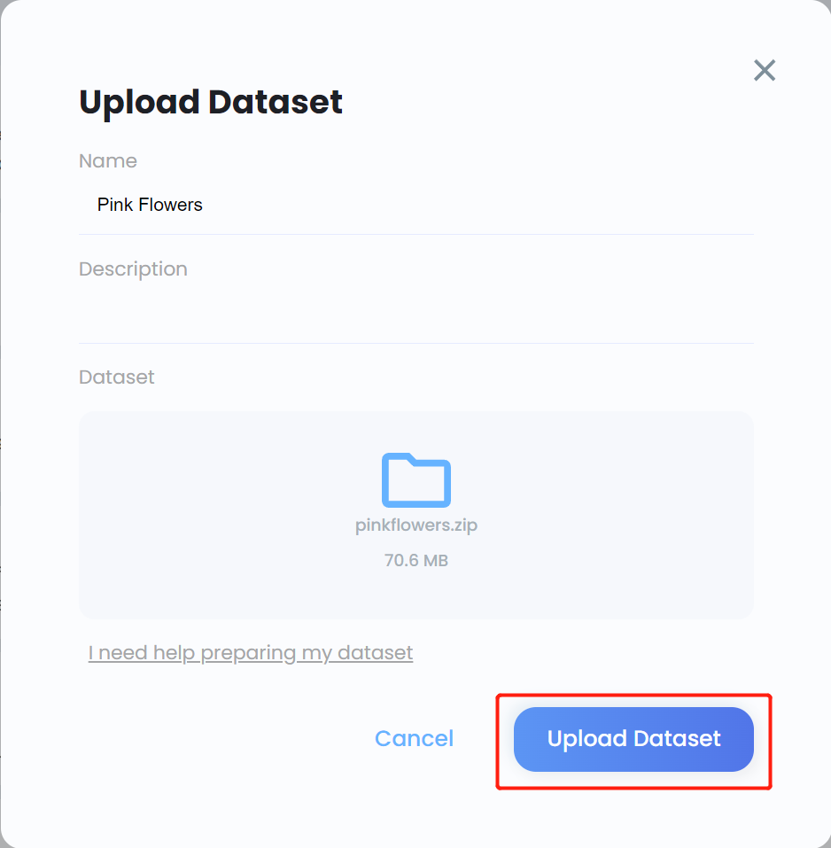
• Step 7. Click on the Datasets tab and click Upload Dataset

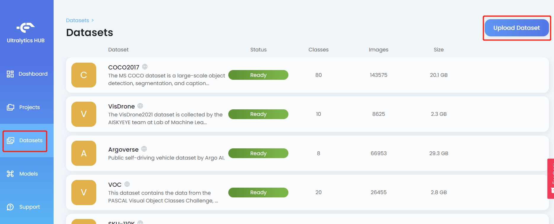
• Step 8. Enter a Name for the dataset, enter a Description if needed, drag and drop the .zip file that we created before under Dataset field and click Upload Dataset

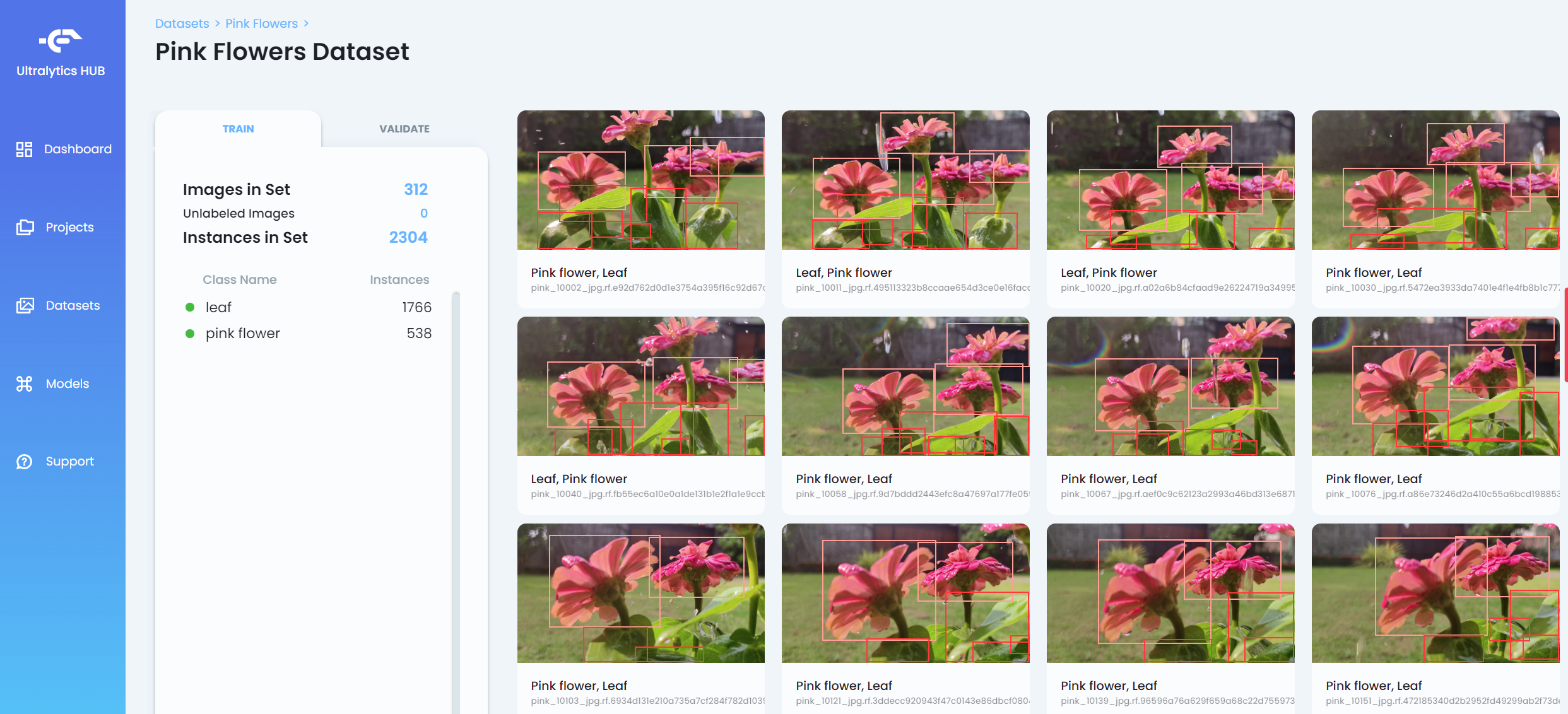
• Step 9. After the datset is uploaded, click on the dataset to view more insights into the dataset

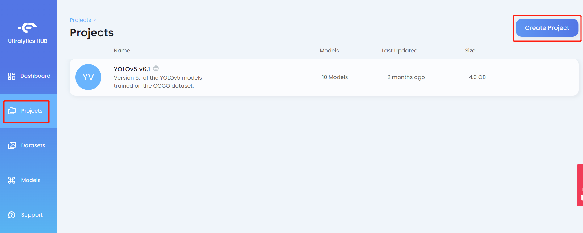
• Step 10. Click on the Projects tab and click Create Project

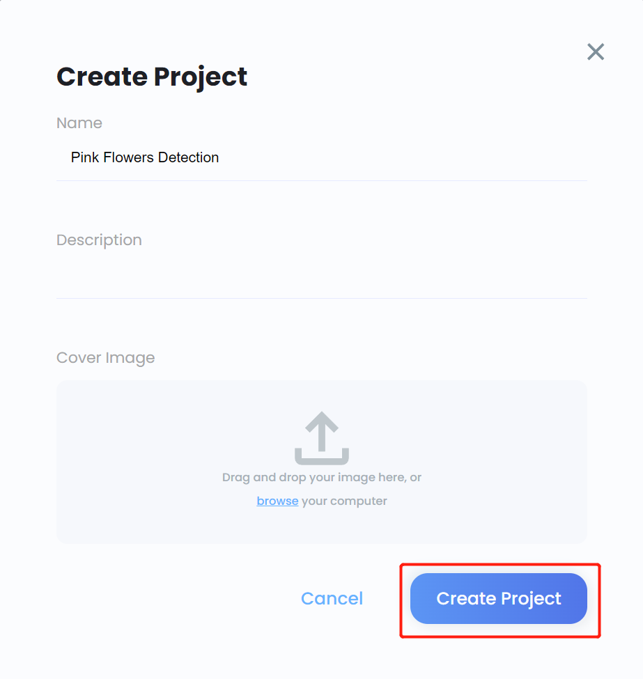
• Step 11. Enter a Name for the project, enter a Description if needed, add a cover image if needed, and click Create Project

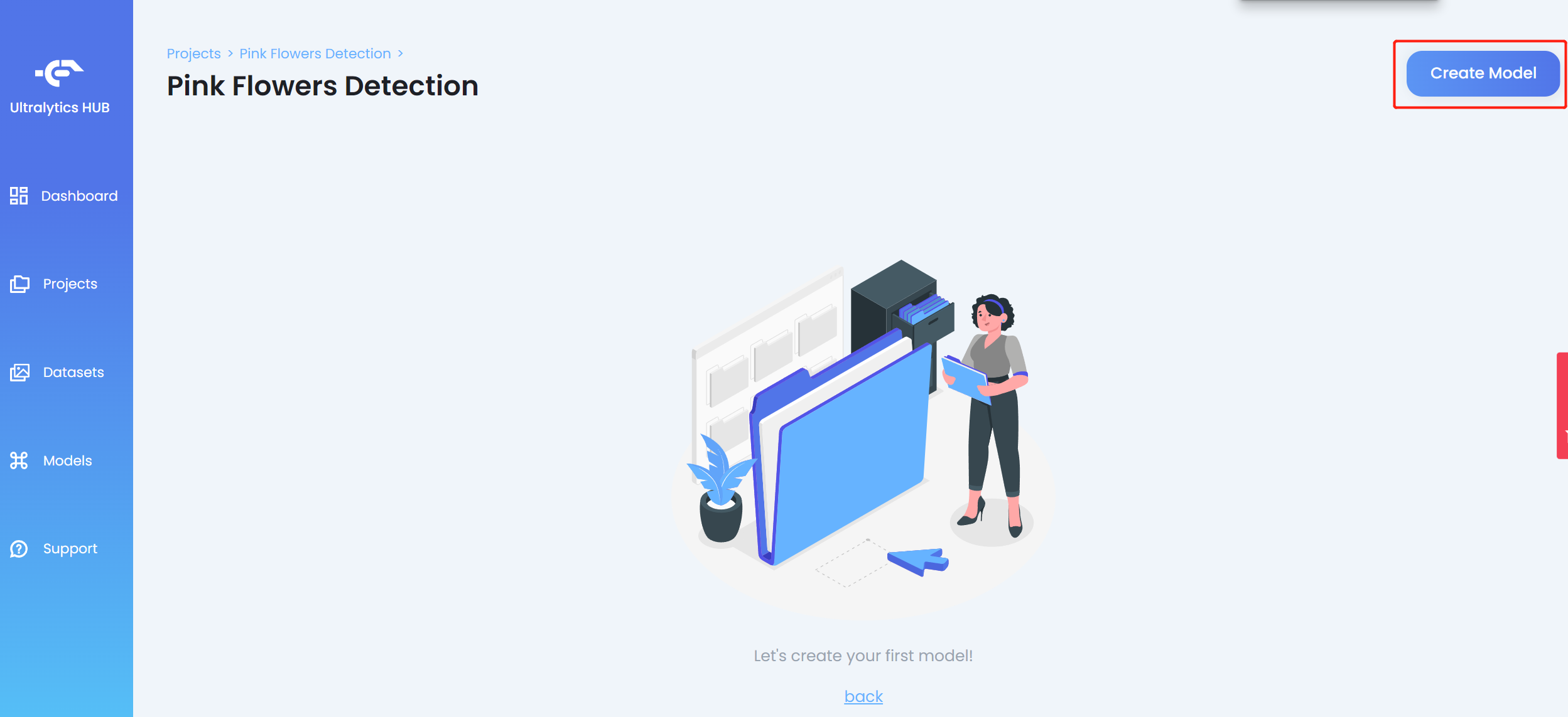
• Step 12. Enter the newly created project and click Create Model

• Step 13. Enter a Model name, choose YOLOv5n as the pretrained model, and click Next

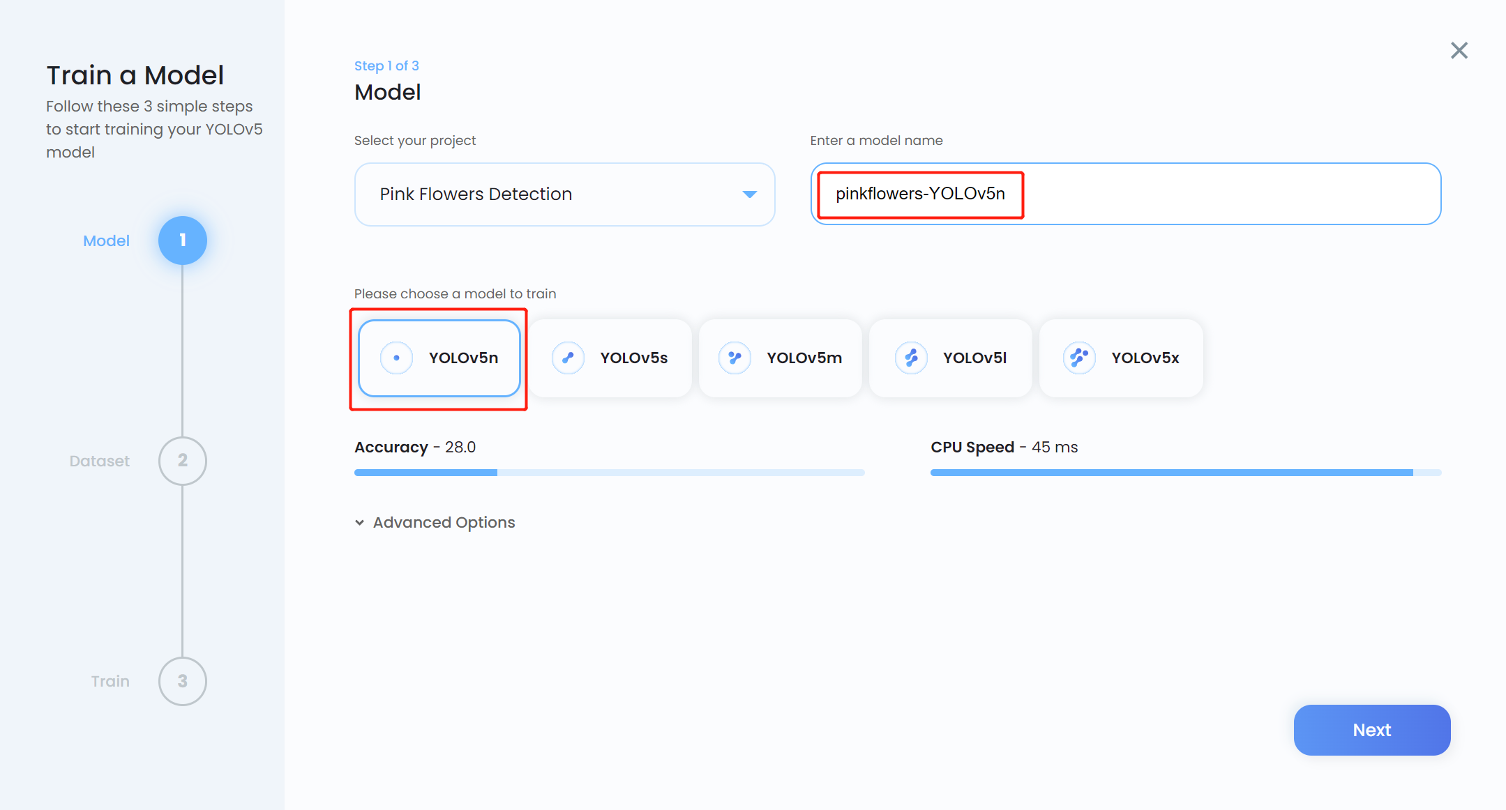
Note: Usually YOLOv5n6 is preferred as the pretrained model because it is suitable to be used for edge devices such as the Jetson platform. However, Ultralytics HUB still does not have the support for it. So we use YOLOv5n which is a slightly similar model.

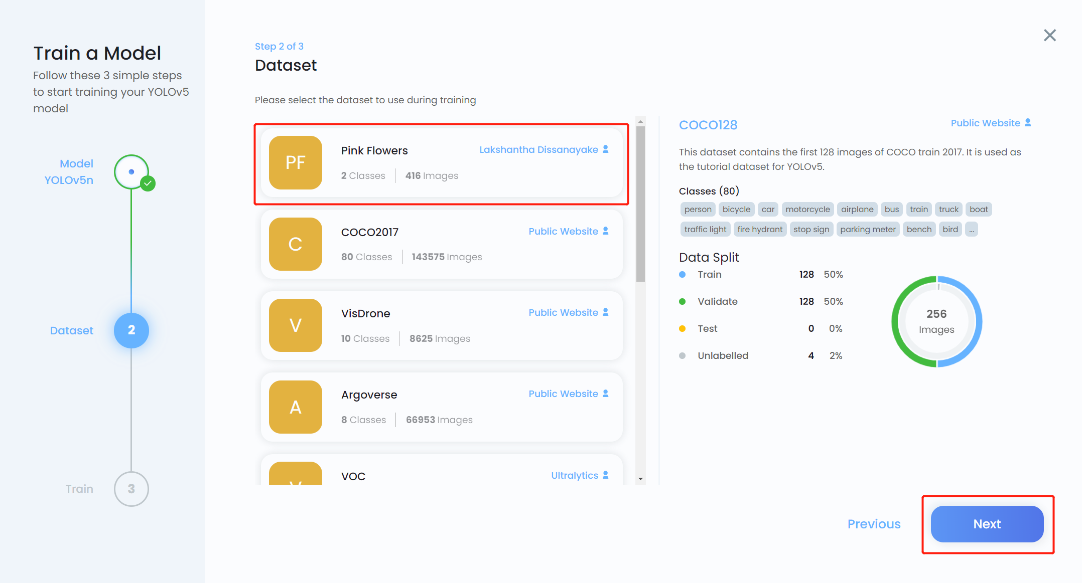
• Step 14. Choose the dataset that we uploaded before and click Next

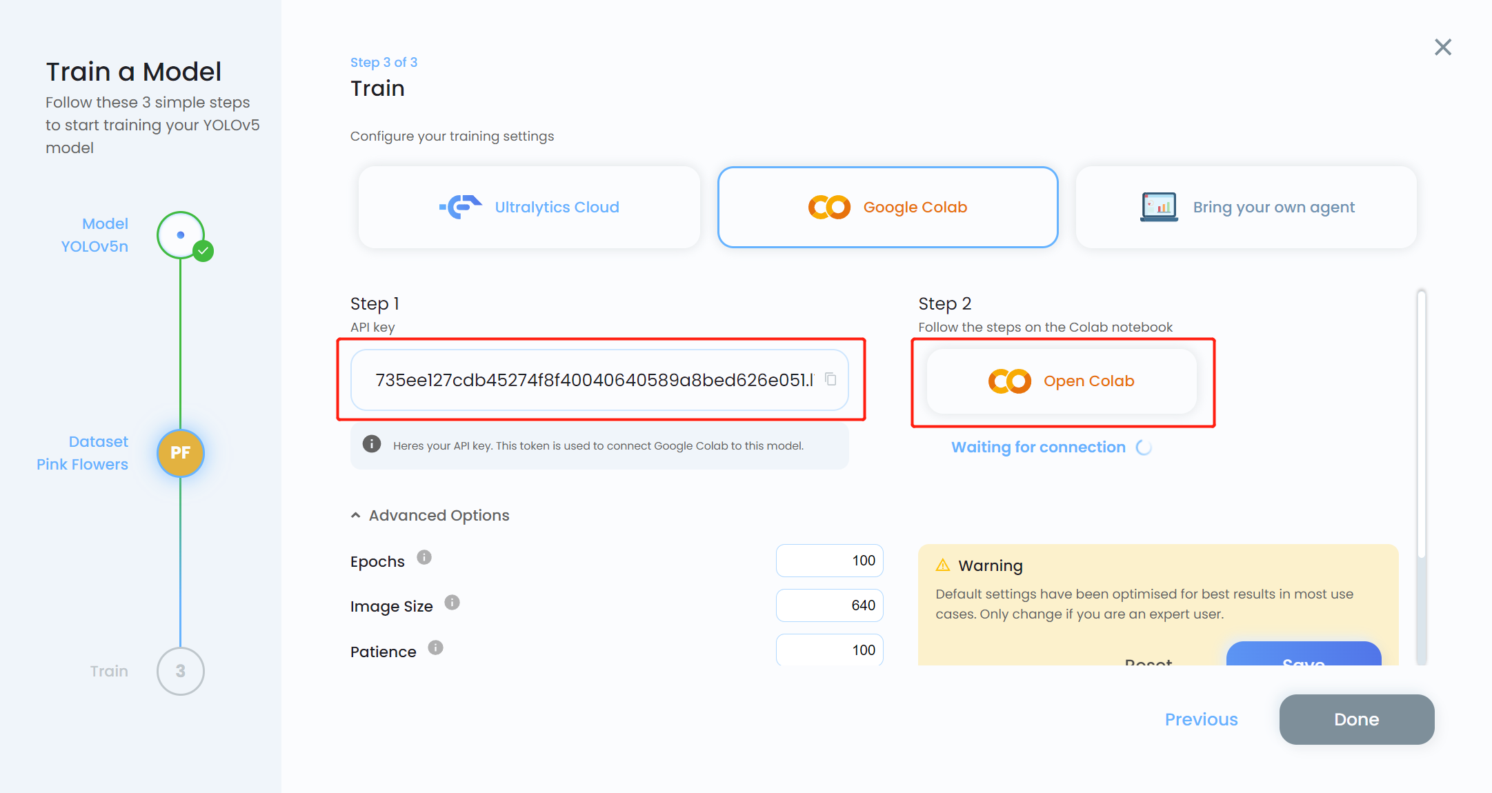
• Step 15. Choose Google Colab as the training platform and click the Advanced Options drop-down menu. Here we can change some settings for training. For example, we will change the number of epochs from 300 to 100 and keep the other settings as they are. Click Save

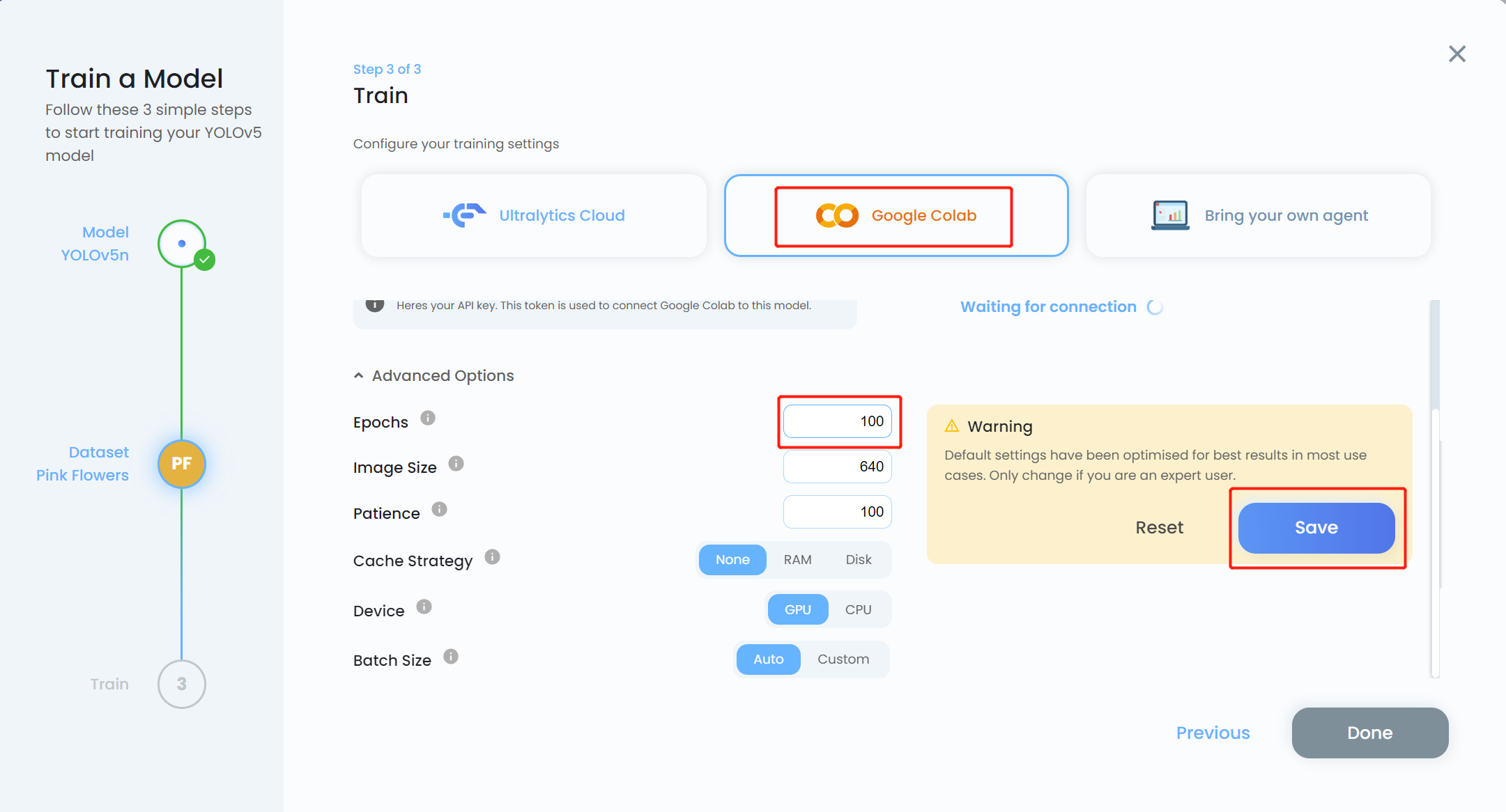
Note: You can also choose Bring your own agent if you are planning to perform local training

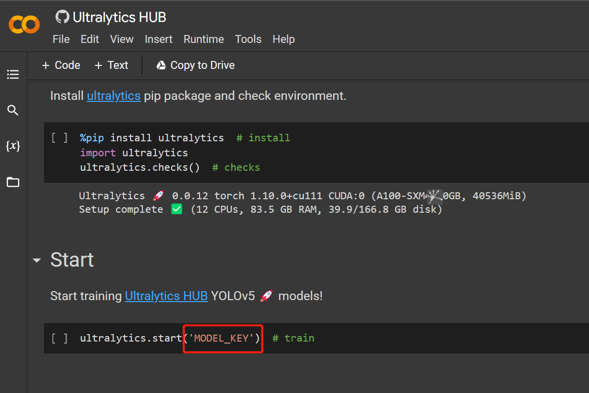
• Step 16. Copy the API key and click Open Colab

• Step 17. Replace MODEL_KEY with the API key that we copied before

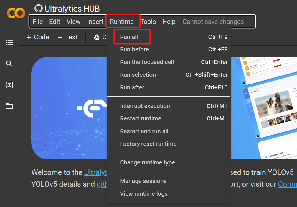
• Step 18. Click Runtime > Rull All to run all the code cells and start the training process

• Step 19. Come back to Ultralytics HUB and click Done when it turns blue. You will also see that Colab shows as Connected.

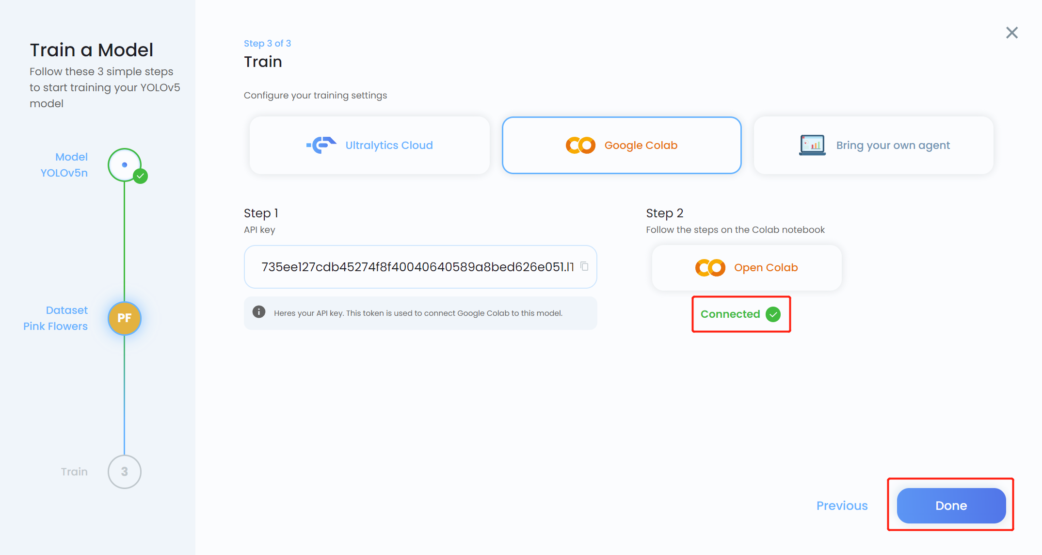
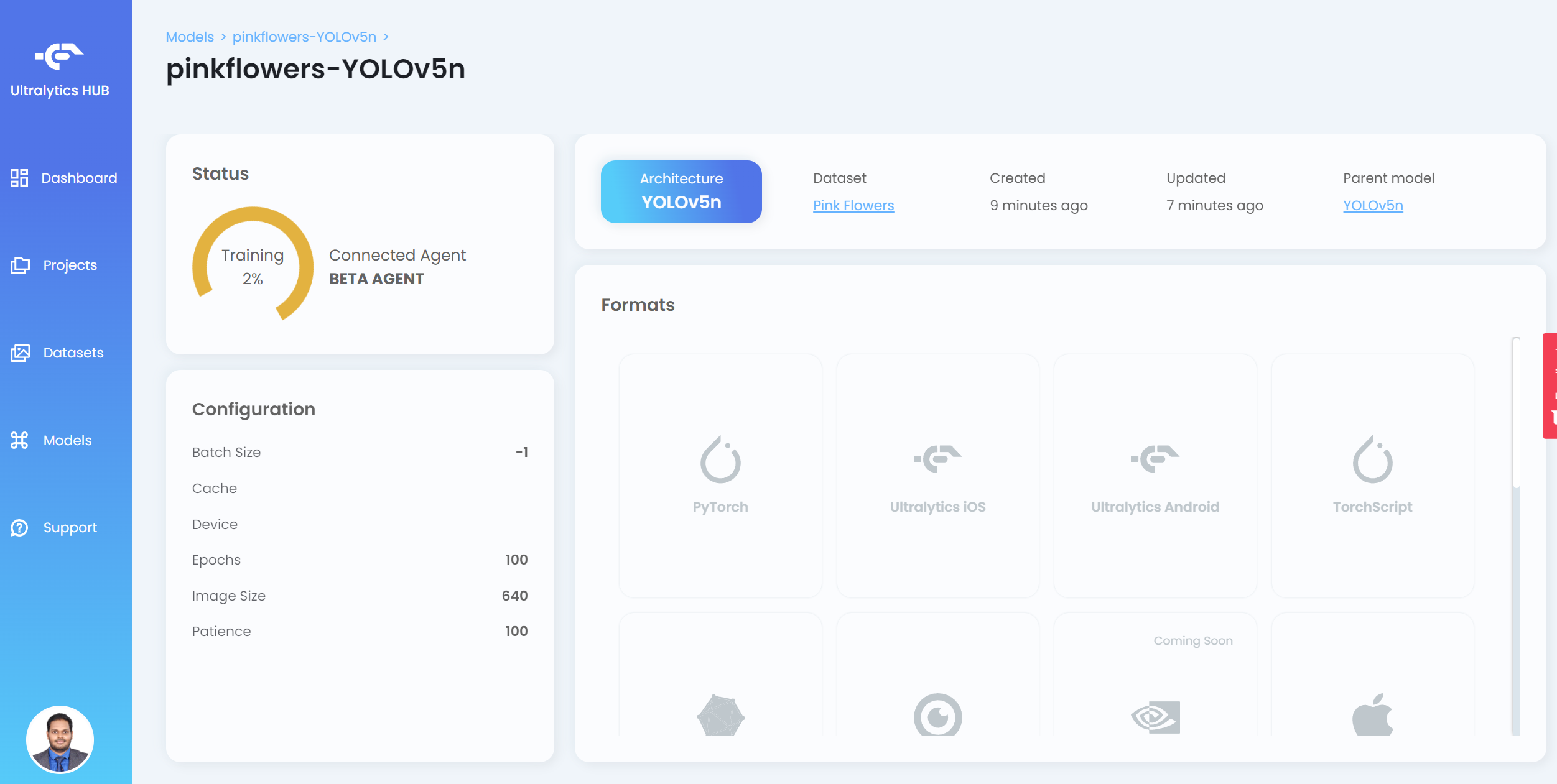
Now you will see the training progress on the HUB

• Step 20. After the training is finished, click PyTorch to download the trained model in PyTorch format. PyTorch is the format that we need in order to perform inference on the Jetson device

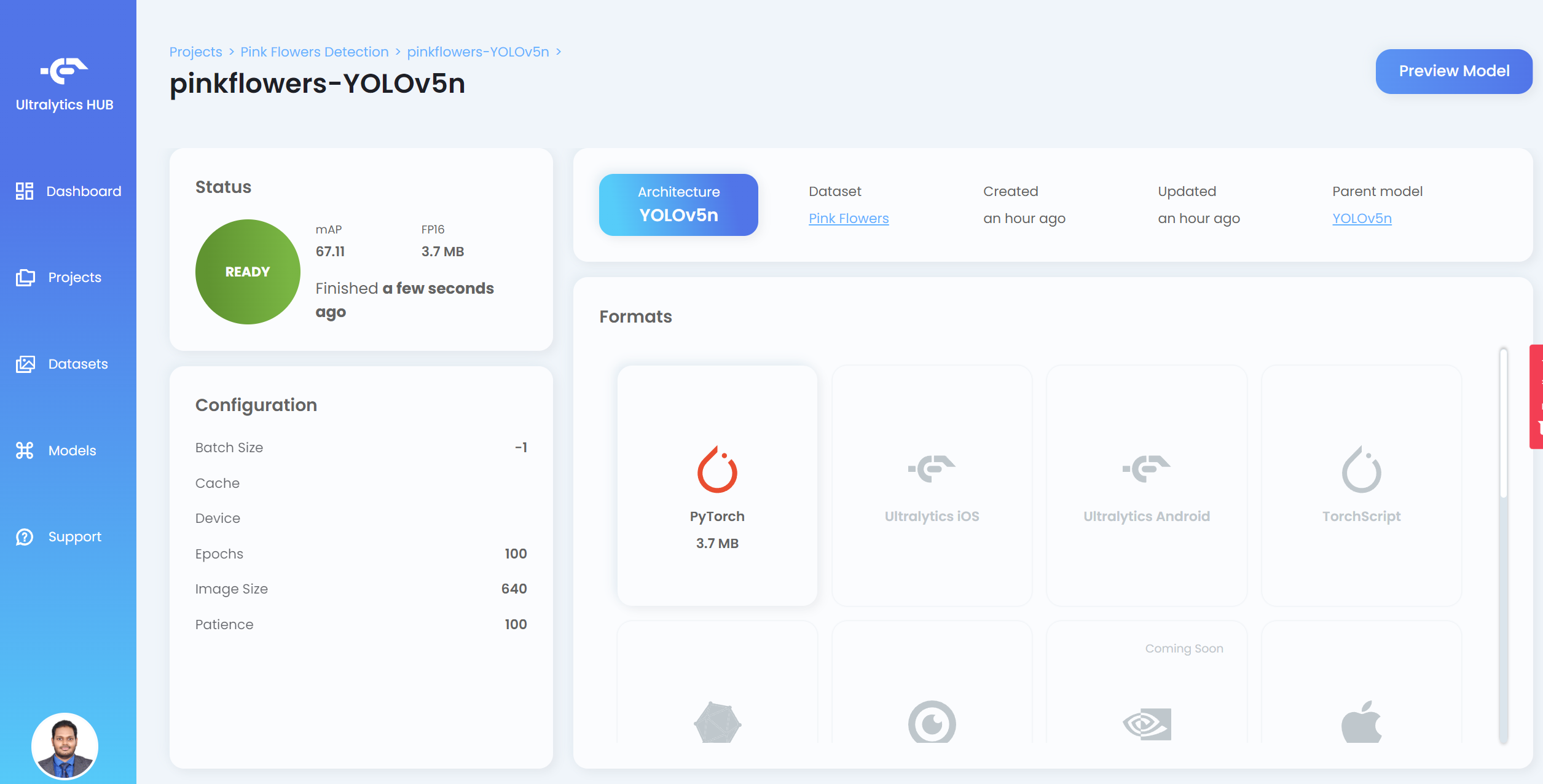
Note: You can also export into other formats as well which are displayed under Formats

If you go back to Google Colab, you can see more details as follows:

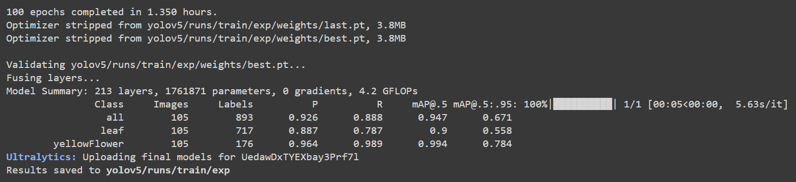
Here the accuracy [email protected] is about 90% and 99.4% for leaf and flower respectively, while the total accuracy [email protected] is about 94.7%.

Use Google Colab with Roboflow api

Here we use a Google Colaboratory environment to perform training on the cloud. Furthermore, we use Roboflow api within Colab to easily download our dataset.

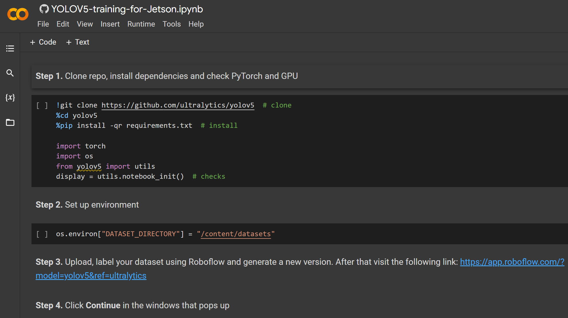
• Step 1. Click here to open an already prepared Google Colab workspace and go through the steps mentioned in the workspace

After the training is done, you will see an output as follows:

Here the accuracy [email protected] is about 91.6% and 99.4% for leaf and flower respectively, while the total accuracy [email protected] is about 95.5%.

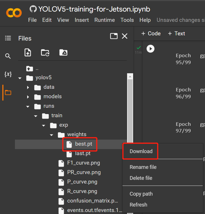
• Step 2. Under Files tab, if you navigate to runs/train/exp/weights, you will see a file called best.pt. This is the generated model from training. Download this file and copy to your Jetson device because this is the model we are going to use later for inferencing on the Jetson device.

Use local PC

Here you can use a PC with a Linux OS for training. We have used an Ubuntu 20.04 PC for this wiki.

• Step 1. Clone the YOLOv5 repo and install requirements.txt in a Python>=3.7.0 environment

git clone https://github.com/ultralytics/yolov5 
cd yolov5
pip install -r requirements.txt

• Step 2. Copy and paste the .zip file that we downloaded before from Roboflow into yolov5 directory and extract it

# example
cp ~/Downloads/pink-flowers.v1i.yolov5pytorch.zip ~/yolov5
unzip pink-flowers.v1i.yolov5pytorch.zip

• Step 3. Open data.yaml file and edit train and val directories as follows

train: train/images
val: valid/images

• Step 4. Execute the following to start training

python3 train.py --data data.yaml --img-size 640 --batch-size -1 --epoch 100 --weights yolov5n6.pt

Since our dataset is relatively small (~500 images), transfer learning is expected to produce better results than training from scratch. Our model was initialized with weights from a pre-trained COCO model, by passing the name of the model (yolov5n6) to the ‘weights’ argument. Here we used yolov5n6 because it is ideal for edge devices. Here the image size is set to 640x640. We use batch-size as -1 because that will automatically determine the best batch size. However, if there is an error which says "GPU memory not enough", choose batch size as 32, or even 16. You can also change epoch according to your preference.

After the training is done, you will see an output as follows:

Here the accuracy [email protected] is about 90.6% and 99.4% for leaf and flower respectively, while the total accuracy [email protected] is about 95%.

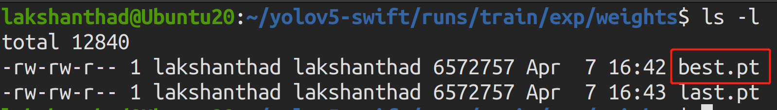
• Step 5. If you navigate to runs/train/exp/weights, you will see a file called best.pt. This is the generated model from training. Copy and paste this file to your Jetson device because this is the model we are going to use later for inferencing on the Jetson device.

Inference on Jetson device

Using TensorRT

Now we will use a Jetson device to perform inference (detect objects) on images with the help of the model generated from our training before. Here we will use NVIDIA TensorRT to increase the inference performance on the Jetson platform

• Step 1. Access the terminal of Jetson device, install pip and upgrade it

sudo apt update
sudo apt install -y python3-pip
pip3 install --upgrade pip

• Step 2. Clone the following repo

git clone https://github.com/ultralytics/yolov5

• Step 3. Open requirements.txt

cd yolov5
vi requirements.txt

• Step 4. Edit the following lines. Here you need to press i first to enter editing mode. Press ESC, then type :wq to save and quit

matplotlib==3.2.2
numpy==1.19.4
# torch>=1.7.0
# torchvision>=0.8.1

Note: We include fixed versions for matplotlib and numpy to make sure there are no errors when running YOLOv5 later. Also, torch and torchvision are excluded for now because they will be installed later.

• Step 5. install the below dependency

sudo apt install -y libfreetype6-dev

• Step 6. Install the necessary packages

pip3 install -r requirements.txt

• Step 7. Install torch

cd ~
sudo apt-get install -y libopenblas-base libopenmpi-dev
wget https://nvidia.box.com/shared/static/fjtbno0vpo676a25cgvuqc1wty0fkkg6.whl -O torch-1.10.0-cp36-cp36m-linux_aarch64.whl
pip3 install torch-1.10.0-cp36-cp36m-linux_aarch64.whl

• Step 8. Install torchvision

sudo apt install -y libjpeg-dev zlib1g-dev
git clone --branch v0.9.0 https://github.com/pytorch/vision torchvision
cd torchvision
sudo python3 setup.py install 

• Step 9. Clone the following repo

cd ~
git clone https://github.com/wang-xinyu/tensorrtx

• Step 10. Copy best.pt file from previous training into yolov5 directory

• Step 11. Copy gen_wts.py from tensorrtx/yolov5 into yolov5 directory

cp tensorrtx/yolov5/gen_wts.py yolov5

• Step 12. Generate .wts file from PyTorch with .pt

cd yolov5
python3 gen_wts.py -w best.pt -o best.wts

• Step 13. Navigate to tensorrtx/yolov5

cd ~
cd tensorrtx/yolov5

• Step 14. Open yololayer.h with vi text editor

vi yololayer.h

• Step 15. Change CLASS_NUM to the number of classes your model is trained. In our example, it is 2

CLASS_NUM = 2

• Step 16. Create a new build directory and navigate inside

mkdir build 
cd build

• Step 17. Copy the previously generated best.wts file into this build directory

cp ~/yolov5/best.wts .

• Step 18. Compile it

cmake ..
make

• Step 19. Serialize the model

sudo ./yolov5 -s [.wts] [.engine] [n/s/m/l/x/n6/s6/m6/l6/x6 or c/c6 gd gw]
#example
sudo ./yolov5 -s best.wts best.engine n6

Here we use n6 because that is recommended for edge devices such as the NVIDIA Jetson platform. However, if you use Ultralytics HUB to set up training, you can only use n because n6 not yet supported by the HUB.

• Step 20. Copy the images that you want the model to detect into a new folder such as tensorrtx/yolov5/images

• Step 21. Deserialize and run inference on the images as follows

sudo ./yolov5 -d best.engine images

Below is a comparison of inference time running on Jetson Nano vs Jetson Xavier NX.

Jetson Nano

Here quantization is set to FP16

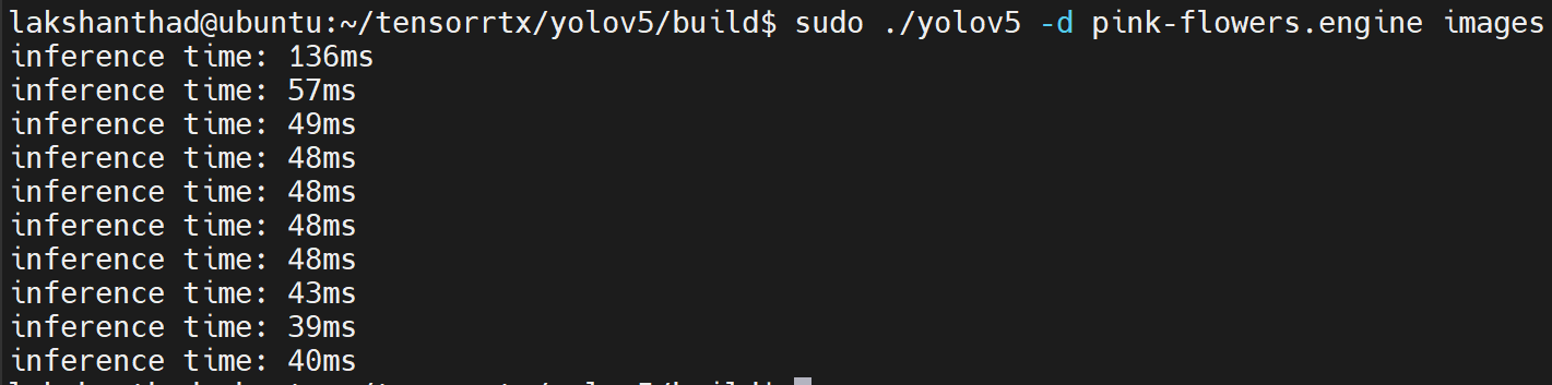
From the above results, we can take the average as about 47ms. Converting this value to frames per second: 1000/47 = 21.2766 = 21fps.

Jetson Xavier NX

Here quantization is set to FP16

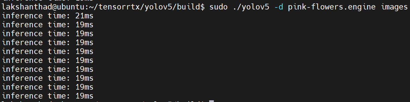
From the above results, we can take the average as about 20ms. Converting this value to frames per second: 1000/20 = 50fps.

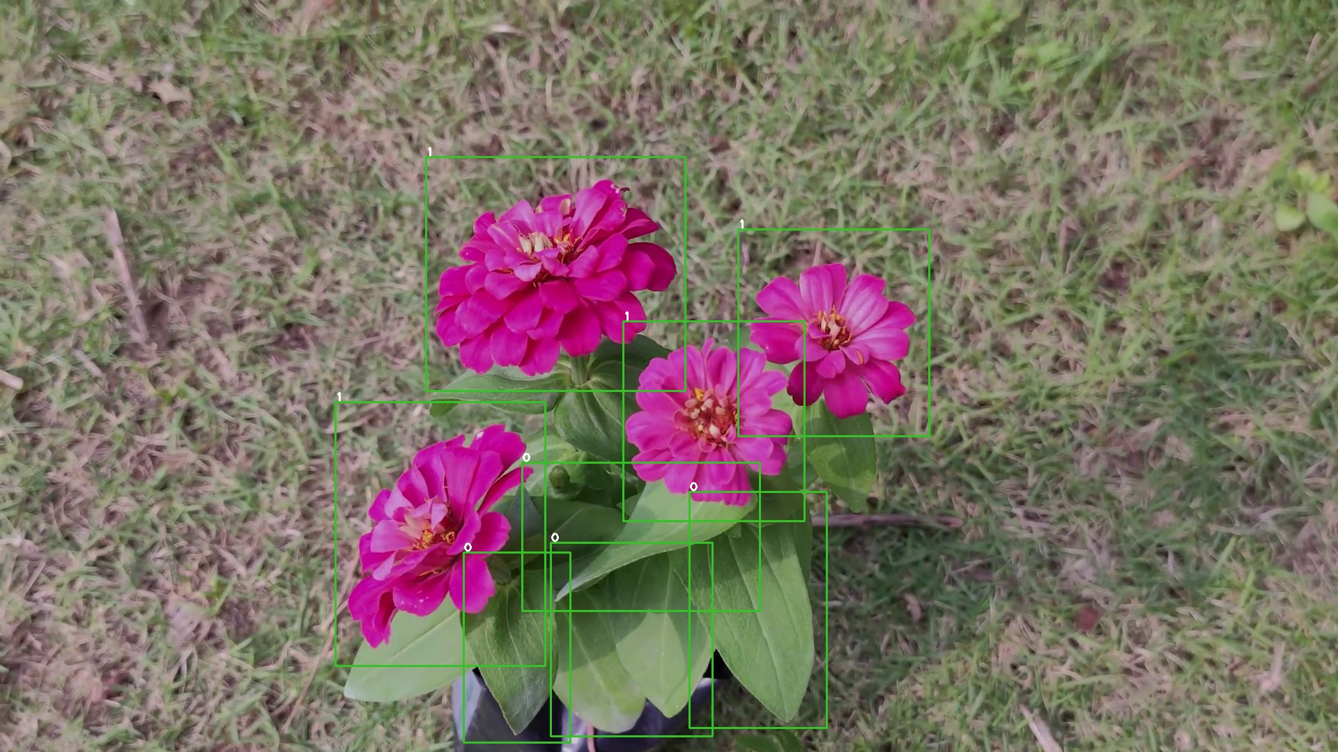
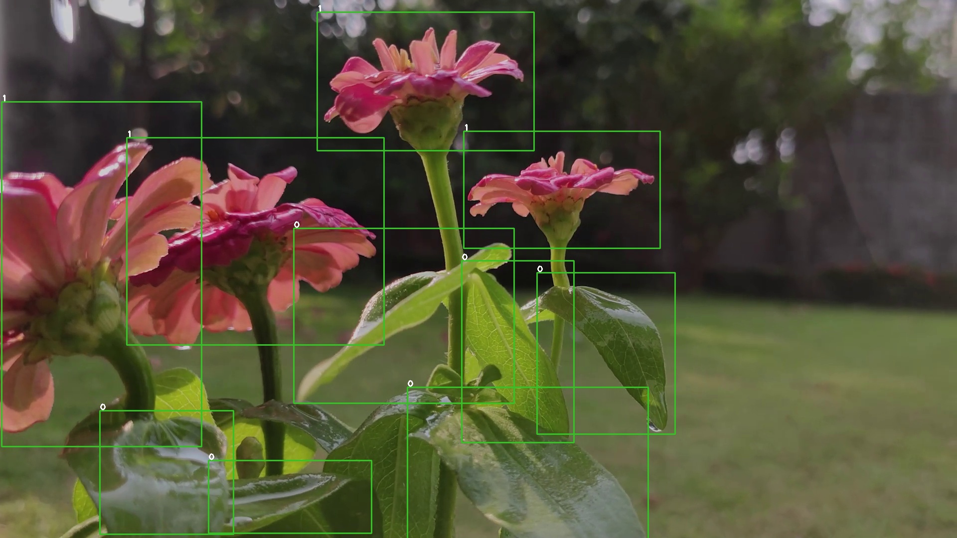
Also, the output images will be as follows with the objects detected:

Using TensorRT and DeepStream SDK

Here we will use NVIDIA TensorRT along with NVIDIA DeepStream SDK to perform inference on a video footage

• Step 1. Make sure you have properly installed all the SDK Components and DeepStream SDK on the Jetson device. (check this wiki for a reference on installation)

Note: It is recommended to use NVIDIA SDK Manager to install all the SDK components and DeepStream SDK

• Step 2. Access the terminal of Jetson device, install pip and upgrade it

sudo apt update
sudo apt install -y python3-pip
pip3 install --upgrade pip

• Step 3. Clone the following repo

git clone https://github.com/ultralytics/yolov5

• Step 4. Open requirements.txt

cd yolov5
vi requirements.txt

• Step 5. Edit the following lines. Here you need to press i first to enter editing mode. Press ESC, then type :wq to save and quit

matplotlib==3.2.2
numpy==1.19.4
# torch>=1.7.0
# torchvision>=0.8.1

Note: We include fixed versions for matplotlib and numpy to make sure there are no errors when running YOLOv5 later. Also, torch and torchvision are excluded for now because they will be installed later.

• Step 6. install the below dependency

sudo apt install -y libfreetype6-dev

• Step 7. Install the necessary packages

pip3 install -r requirements.txt

• Step 8. Install torch

cd ~
sudo apt-get install -y libopenblas-base libopenmpi-dev
wget https://nvidia.box.com/shared/static/fjtbno0vpo676a25cgvuqc1wty0fkkg6.whl -O torch-1.10.0-cp36-cp36m-linux_aarch64.whl
pip3 install torch-1.10.0-cp36-cp36m-linux_aarch64.whl

• Step 9. Install torchvision

sudo apt install -y libjpeg-dev zlib1g-dev
git clone --branch v0.9.0 https://github.com/pytorch/vision torchvision
cd torchvision
sudo python3 setup.py install 

• Step 10. Clone the following repo

cd ~
git clone https://github.com/marcoslucianops/DeepStream-Yolo

• Step 11. Copy gen_wts_yoloV5.py from DeepStream-Yolo/utils into yolov5 directory

cp DeepStream-Yolo/utils/gen_wts_yoloV5.py yolov5

• Step 12. Inside the yolov5 repo, download pt file from YOLOv5 releases (example for YOLOv5s 6.1)

cd yolov5
wget https://github.com/ultralytics/yolov5/releases/download/v6.1/yolov5s.pt

• Step 13. Generate the cfg and wts files

python3 gen_wts_yoloV5.py -w yolov5s.pt

Note: To change the inference size (defaut: 640)

-s SIZE
--size SIZE
-s HEIGHT WIDTH
--size HEIGHT WIDTH

Example for 1280:
-s 1280
or
-s 1280 1280

• Step 14. Copy the generated cfg and wts files into the DeepStream-Yolo folder

cp yolov5s.cfg ~/DeepStream-Yolo
cp yolov5s.wts ~/DeepStream-Yolo

• Step 15. Open the DeepStream-Yolo folder and compile the library

cd ~/DeepStream-Yolo
# For DeepStream 6.1
CUDA_VER=11.4 make -C nvdsinfer_custom_impl_Yolo
# For DeepStream 6.0.1 / 6.0
CUDA_VER=10.2 make -C nvdsinfer_custom_impl_Yolo

• Step 16. Edit the config_infer_primary_yoloV5.txt file according to your model

[property]
...
custom-network-config=yolov5s.cfg
model-file=yolov5s.wts
...

• Step 17. Edit the deepstream_app_config file

...
[primary-gie]
...
config-file=config_infer_primary_yoloV5.txt

• Step 18. Run the inference

deepstream-app -c deepstream_app_config.txt

The above result is running on Jetson Xavier NX with FP32 and YOLOv5s 640x640. We can see that the FPS is around 30.

INT8 Calibration

If you want to use INT8 precision for inference, you need to follow the steps below

• Step 1. Install OpenCV

sudo apt-get install libopencv-dev

• Step 2. Compile/recompile the nvdsinfer_custom_impl_Yolo library with OpenCV support

cd ~/DeepStream-Yolo
# For DeepStream 6.1
CUDA_VER=11.4 OPENCV=1 make -C nvdsinfer_custom_impl_Yolo
# For DeepStream 6.0.1 / 6.0
CUDA_VER=10.2 OPENCV=1 make -C nvdsinfer_custom_impl_Yolo

• Step 3. For COCO dataset, download the val2017, extract, and move to DeepStream-Yolo folder

• Step 4. Make a new directory for calibration images

mkdir calibration

• Step 5. Run the following to select 1000 random images from COCO dataset to run calibration

for jpg in $(ls -1 val2017/*.jpg | sort -R | head -1000); do \
    cp ${jpg} calibration/; \
done

Note: NVIDIA recommends at least 500 images to get a good accuracy. On this example, 1000 images are chosen to get better accuracy (more images = more accuracy). Higher INT8_CALIB_BATCH_SIZE values will result in more accuracy and faster calibration speed. Set it according to you GPU memory. You can set it from head -1000. For example, for 2000 images, head -2000. This process can take a long time.

• Step 6. Create the calibration.txt file with all selected images

realpath calibration/*jpg > calibration.txt

• Step 7. Set environment variables

export INT8_CALIB_IMG_PATH=calibration.txt
export INT8_CALIB_BATCH_SIZE=1

• Step 8. Update the config_infer_primary_yoloV5.txt file

From

...
model-engine-file=model_b1_gpu0_fp32.engine
#int8-calib-file=calib.table
...
network-mode=0
...

To

...
model-engine-file=model_b1_gpu0_int8.engine
int8-calib-file=calib.table
...
network-mode=1
...

• Step 9. Run the inference

deepstream-app -c deepstream_app_config.txt

The above result is running on Jetson Xavier NX with INT8 and YOLOv5s 640x640. We can see that the FPS is around 60.

Benchmark results

The following table summarizes how different models perform on Jetson Xavier NX.

Model Name	Precision	Inference Size	Inference Time (ms)	FPS
YOLOv5s	FP32	320x320	16.66	60
	FP32	640x640	33.33	30
	INT8	640x640	16.66	60
YOLOv5n	FP32	640x640	16.66	60

Comparison between using public datasets and custom datasets

Now we will compare the difference between the number of training samples and training time when using public datasets and your own custom datasets

Number of training samples

Custom dataset

In this wiki, we collected our plant dataset as a video first and then converted the video into a series of images using Roboflow. Here we obtained 542 images which is a very small dataset when compared with public datasets.

Public dataset

Public datasets such as Pascal VOC 2012 and Microsoft COCO 2017 dataset have around 17112 and 121408 Images repectively.

Pascal VOC 2012 dataset

Microsoft COCO 2017 dataset

Training time

Local training

The training was done on an NVIDIA GeForce GTX 1660 Super Graphics Card with 6GB memory

Custom dataset with local training

540 images dataset

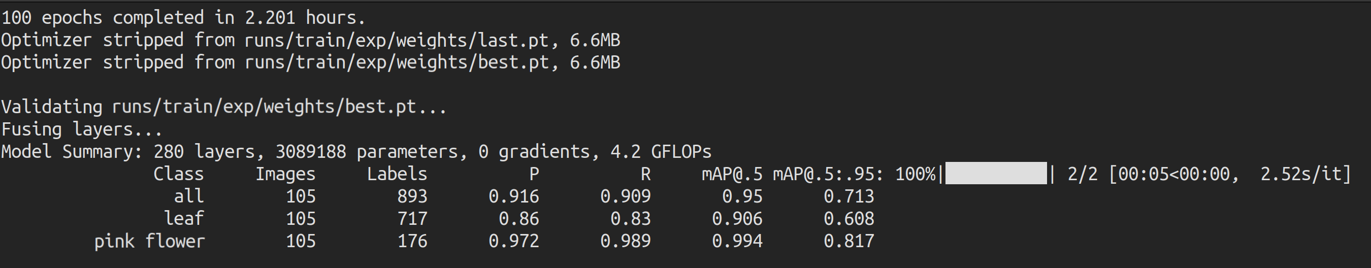
According to the local training we performed before for the plants, we obtained the following results

Here it took only 2.2 hours run 100 epochs. This is comparatively faster than training using public datasets.

240 images dataset

We reduced the dataset to 240 images and performed training again and obtained the following results

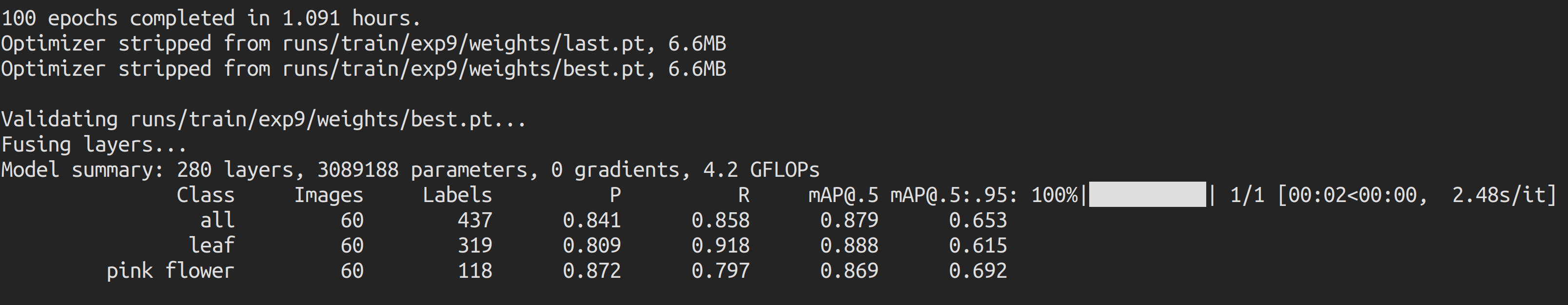
Here it took only about 1 hour run 100 epochs. This is comparatively faster than training using public datasets.

Pascal VOC 2012 dataset with local training

We used a Pascal VOC 2012 dataset for the training in this scenario while keeping the same training parameters. We found that it was taking about 50 minutes (0.846 hours * 60) to run 1 epoch, and therefore we stopped the training on 1 epoch.

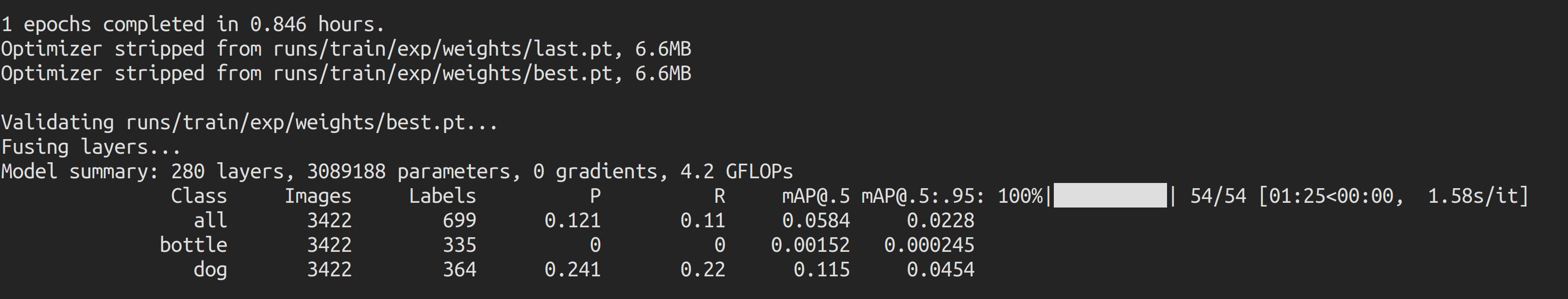
If we calculate the training time for 100 epochs, it would take about 50 * 100 minutes = 5000 minutes = 83 hours which is much longer than the training time for the custom dataset.

Microsoft COCO 2017 Dataset with local training

We used a Microsoft COCO 2017 dataset for the training in this scenario while keeping the same training parameters. We found that it was estimated to take about 7.5 hours to run 1 epoch, and therefore we stopped the training before 1 epoch was finished.

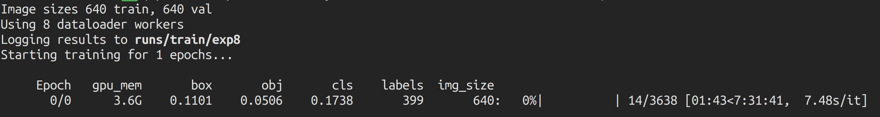
If we calculate the training time for 100 epochs, it would take about 7.5 hours * 100 = 750 hours which is much longer than the training time for the custom dataset.

Google Colab training

The training was done on an NVIDIA Tesla K80 Graphics Card with 12GB memory

Custom dataset

540 images dataset

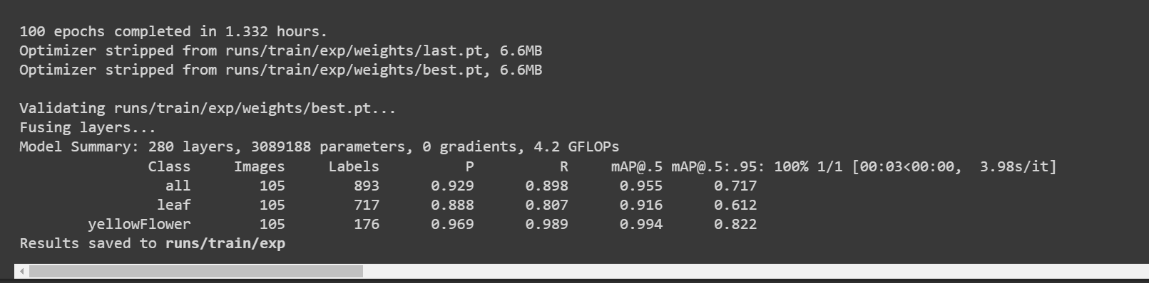
According to the Google Colab training we performed before for the plants with 540 images, we obtained the following results

Here it took only about 1.3 hours run 100 epochs. This is also comparatively faster than training using public datasets.

240 images dataset

We reduced the dataset to 240 images and performed training again and obtained the following results

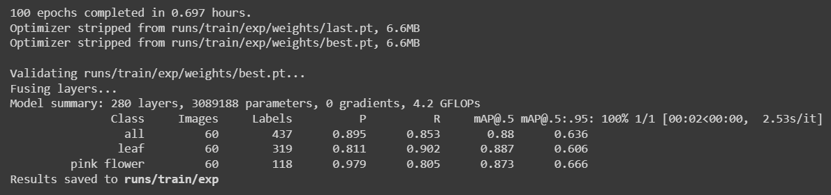
Here it took only about 42 minutes (0.697 hours * 60) run 100 epochs. This is comparatively faster than training using public datasets.

Pascal VOC 2012 dataset with Google Colab training

We used a Pascal VOC 2012 dataset for the training in this scenario while keeping the same training parameters. We found that it was taking about 9 minutes (0.148 hours * 60) to run 1 epoch, and therefore we stopped the training on 1 epoch.

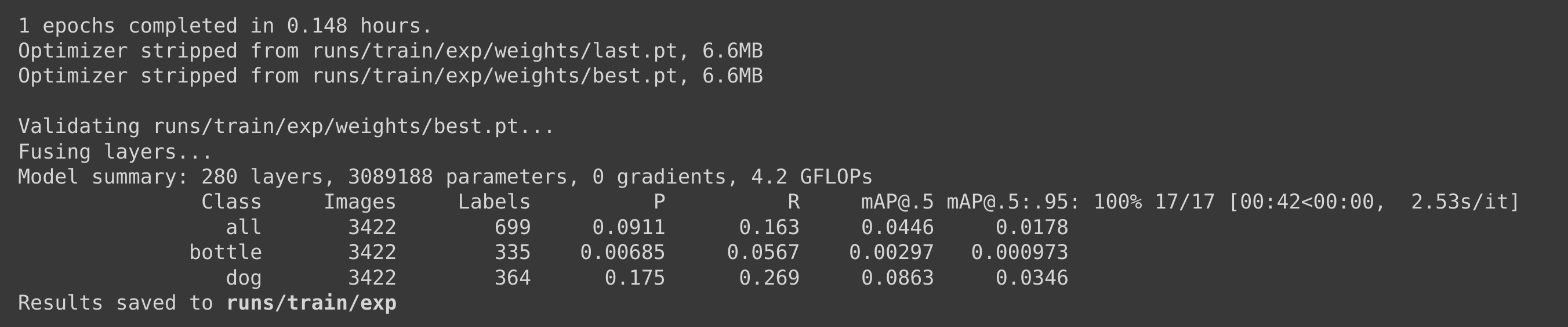
If we calculate the training time for 100 epochs, it would take about 9 * 100 minutes = 900 minutes = 15 hours which is much longer than the training time for the custom dataset.

Microsoft COCO 2017 Dataset with Google Colab training

We used a Microsoft COCO 2017 dataset for the training in this scenario while keeping the same training parameters. We found that it was estimated to take about 1.25 hours to run 1 epoch, and therefore we stopped the training before 1 epoch was finished.

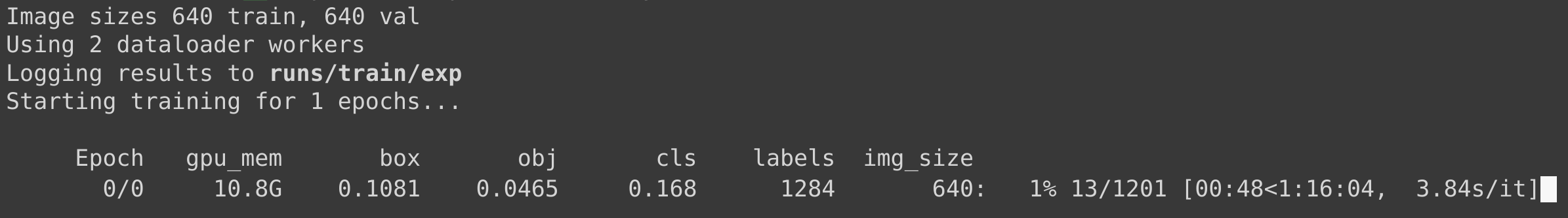
If we calculate the training time for 100 epochs, it would take about 1.25 hours * 100 = 125 hours which is much longer than the training time for the custom dataset.

Number of training samples and training time summary

Dataset	Number of training samples	Training time on Local PC (GTX 1660 Super)	Training time on Google Colab (NVIDIA Tesla K80)
Custom	542	2.2 hours	1.3 hours
	240	1 hour	42 minutes
Pascal VOC 2012	17112	83 hours	15 hours
Microsoft COCO 2017	121408	750 hours	125 hours

Pretrained checkpoints comparison

You can learn more about pretrained checkpoints from the table below. Here we have highlighted our scenario when trained with Google Colab and inference done on Jetson Nano and Jetson Xavier NX with YOLOv5n6 as the pretrained checkpoint.

Model	size (pixels)	mAPval 0.5:0.95	mAPval 0.5	Speed CPU b1 (ms)	Speed V100 b1 (ms)	Speed V100 b32 (ms)	Speed Jetson Nano FP16 (ms)	Speed Jetson Xavier NX FP16 (ms)	params (M)	FLOPs @640 (B)
YOLOv5n	640	28.0	45.7	45	6.3	0.6			1.9	4.5
YOLOv5s	640	37.4	56.8	98	6.4	0.9			7.2	16.5
YOLOv5m	640	45.4	64.1	224	8.2	1.7			21.2	49.0
YOLOv5l	640	49.0	67.3	430	10.1	2.7			46.5	109.1
YOLOv5x	640	50.7	68.9	766	12.1	4.8			86.7	205.7
YOLOv5n6	640	71.7	95.5	153	8.1	2.1	47	20	3.1	4.6
YOLOv5s6	1280	44.8	63.7	385	8.2	3.6			12.6	16.8
YOLOv5m6	1280	51.3	69.3	887	11.1	6.8			35.7	50.0
YOLOv5l6	1280	53.7	71.3	1784	15.8	10.5			76.8	111.4
YOLOv5x6 + [TTA]	1280 1536	55.0 55.8	72.7 72.7	3136 -	26.2 -	19.4 -			140.7 -	209.8 -

Reference: YOLOv5 GitHub

Bonus Applications

Since all the steps that we explained above are common for any type of object detection application, you only need to change the dataset for your own object detection application!

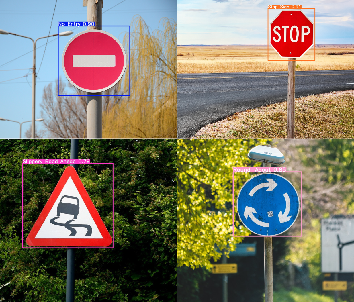
Road signs detection

Here we used the road signs dataset from Roboflow and performed inference on NVIDIA Jetson!

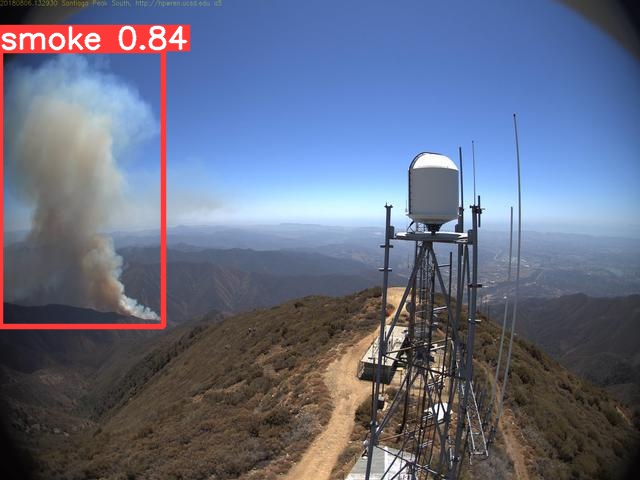
Wildfire smoke detection

Here we used wildfire smoke dataset from Roboflow and performed inference on NVIDIA Jetson!

Resources

• [Web Page] YOLOv5 Documentation

• [Web Page] Ultralytics HUB

• [Web Page] Roboflow Documentation

Tech Support & Product Discussion

Thank you for choosing our products! We are here to provide you with different support to ensure that your experience with our products is as smooth as possible. We offer several communication channels to cater to different preferences and needs.